Guest essay by Javier

Solar cycle 24 is ending and we are approaching a time of minimal solar activity between solar cycles 24 and 25, known as a solar minimum. Despite claims that we understand how the Sun works, our solar predictive skills are still wanting, and the Sun continues to be full of surprises.

The surprising 2008 solar minimum

Solar scientists did not pay much attention to the early warning signs that the Sun was behaving differently during solar cycle 23 (SC23), and to most the surprise came when the expected solar minimum failed to show up in 2006. The SC23-24 minimum took place two years later (Dec 2008, according to SIDC), and despite showing only a tiny difference in total solar irradiation compared to previous minima of the space age, it displayed significantly reduced solar wind speed and density, extreme-UV flux was 10% reduced, the polar fields were 50% smaller, and the interplanetary magnetic field strength was 30% below past minima. In response to the changes in the Sun, the density of the Earth thermosphere dropped 20% lower than in previous minima. In 2007 Svalgaard & Cliver proposed a floor to the interplanetary magnetic field at 1 AU in the ecliptic plane of 4.6 nT based upon 130 years of data. This floor has implications for the solar wind during grand minima. After the solar minimum, in 2011, Cliver & Ling were forced to revise down the floor to 2.8 nT, a 40 percent reduction! The SC23-24 minimum was truly shocking to solar scientists, showing them how little they knew of what happens to the Sun when it becomes very inactive. And it was just a centennial-type solar minimum, not a grand-type solar minimum.

We are now approaching the SC24-25 solar minimum, and again the Sun’s behavior surprises us. Or doesn’t it? On April 26, NOAA informed us that “current solar cycle 24 is declining more quickly than forecast.”

The rapid decline in solar activity plus the appearance of the first SC25 spots suggest that SC24 could be both a low-activity and short solar cycle. This would not be unusual since cycle length and cycle activity do not correlate significantly (figure 1).

Figure 1. Solar cycle activity versus cycle length. The activity is the sum of the monthly sunspots for the entire cycle. SC24 (in red) is still provisional, and the dashed arrow indicates a possible path it might follow until the solar minimum takes place. The Dalton Minimum (purple), Gleissberg Minimum (blue), and Modern Maximum (orange) cycles are indicated. The Modern Maximum is a period of seven consecutive high activity solar cycles in a period that coincides with high anthropogenic CO₂ emissions and global warming (1935-2005). The longest such stretch of high solar activity known.

We have read at WUWT both that the solar minimum may have already happened, or that it might take place in 2026. None of these opinions appear to be based on much fact, so we should examine the question in more detail.

Defining a solar minimum

While intuitively we all understand that a solar minimum is the period of time that shows the least amount of solar activity between two cycles, how the solar minimum is defined can make a difference of months in the date of the minimum. Harvey & White reviewed in 1999 the different methods used to define a solar minimum:

“In addition to the time of a minimum in the smoothed sunspot number, historically the basis for the determination of the time of cycle minimum since 1889 includes the time of the minimum or minima in the monthly averaged sunspot number, the number of spotless days, the start and end times of the minimum phase, the number of regions belonging to the outgoing (old) and incoming (new) cycles, and the use of different smoothing windows.”

Some of them are shown in table 1 from Harvey & White 1999.

Table 1. Illustration of the problems of defining the solar minimum. Column 2 shows the date given by prominent researchers. Columns 3-7 give the date of the minimum activity as calculated by different methods. Source: Harvey & White 1999.

According to Harvey & White 1999, the SC22-23 minimum should be placed, based on an average of five parameters, on Sep. 1996. The Solar Influences Data Center (SIDC), responsible for the World Data Center for Sunspot Index and Long-term Solar Observations (WDC-SILSO) at the Royal Observatory of Belgium (Brussels), uses the following 13-month smoothing formula:

R_s= (0.5 R_m±6 + R_m±5 + R_m±4 + R_m±3 + R_m±2 + R_m±1 + R_m) / 12 …….[1]

Where R_s is the smoothed sunspot number and R_m the monthly sunspot number for the central month. The end months in the average are given half weight.

This formula produces Aug. 1996 for the SC22-23 minimum so, despite being very simple, the result is generally quite close to more complex calculations.

This formula requires that at least 7 months have passed since the minimum and produces a 6-month delay in the calculation of monthly solar activity. For this article, I wanted to reduce this delay without compromising accuracy too much, so I have used the following 9-month smoothing formula with a more skewed weighting:

R_s= (R_m±4 + 3 R_m±3 + 5 R_m±2 + 7 R_m±1 + 10 R_m) / 42 …….[2]

Figure 2 shows the result of smoothing [2] compared to SIDC smoothing [1].

Figure 2. Sunspot smoothing used in this article [2] (grey line) compared to the SIDC smoothing [1] (black line).

Have we reached already the SC24-25 minimum?

The answer is almost certainly not. We can base this answer on two kinds of data. The first is the number of spotless days. Astronomers have been counting the number of spotless days since 1818, and this number in the current minimum, as of first of June is 198 (Figure 3). As the solar minimum usually takes place after at least half of the spotless days in a minimum have taken place (the rising phase of the cycle is usually faster than the declining phase), that would imply that this minimum should have less than 400 spotless days if it ended now. Such a low number has only taken place in minima between very active solar cycles during the Modern Maximum in solar activity (1935-2005). Given that SC24 has been a low-activity cycle we should expect 200-300 spotless days more before the minimum is reached, and that is about a year of very low solar activity.

Figure 3. Number of spotless days per cycle minimum transition (red) and the yearly international sunspot number (S_n, inverted, green) since 1818. Note that, in general, a low amplitude cycle is preceded by a solar cycle transition with a high number of spotless days, and vice versa. The blue dot to the lower right represents the number of spotless days (198) for the current cycle transition. Source: WDC-SILSO.

The second kind of data are the number of SC25 sunspot groups. SC25 sunspots have been appearing since December 2016, but the solar minimum is usually located at the time when the numbers of SC24 and SC25 sunspot groups are even, or slightly later. As it can be seen in figure 4, we aren’t there yet.

Figure 4. Monthly number of sunspot groups (having received a NOAA number) from SC24 (black) and from SC25 (white) since 2016. The red curve represents the smoothed monthly international sunspot number. Source: Solar-Terrestrial Centre of Excellence.

When is it most likely that the SC24-25 minimum will occur?

Most of the analyses I have seen have one problem. They only look at a subset of solar cycles, and the space-age records are biased by the high activity of the Modern Maximum. I have been inspired particularly by Belgian astronomer Jan Janssens’ SC24 tracking webpage. Using the smoothing filter [2], and following Janssens, I have defined the starting point of the analysis of each minimum as the last month that showed ≥ 30 monthly smoothed sunspots before the minimum. In figure 5 I have represented the number of months it took for each transition from that starting point to reach its solar minimum (lowest smoothed monthly sunspot number or central month when several consecutive zero values).

Figure 5. Distribution of solar cycles by the time it takes them to go from ≥ 30 monthly smoothed sunspots to their solar minimum. The distribution shows a clear difference between cycles with less than 14 months and cycles with more than 19 months.

The distribution is clearly bimodal. 13 transitions took between 8 and 14 months to reach the solar minimum from ≥ 30 smoothed sunspots (short or fast solar minima), while 11 transitions took between 19 and 44 months (long solar minima). For the SC24-25 transition the value of 30 smoothed monthly sunspots was reached in October 2016, 20 months ago as of this writing. For graphical convenience I have divided the long solar minima in two groups. The medium solar minima (19-32 months), and the slow solar minima (38-44 months).

Figure 6. Comparison of the present solar minimum (in red) to the group with fast (short) solar minima.

The present solar minimum does not belong to the group characterized by short solar minima. The sunspot number is falling too abruptly, and the solar minimum should have been hit by December 2017 to belong to the group. As of June (corresponding to January 2018 smoothed data) the smoothed sunspot number is still decreasing and given the evolution it will decrease again next month.

Figure 7. Comparison of the present solar minimum (in red) to the group with medium speed solar minima.

The present solar minimum could belong to the medium group. This group includes solar cycle minima from the Dalton and Gleissberg extended minima, but also the unusual 1986 SC21-22 minimum. If SC24-25 belongs to this group the minimum should take place between May 2018 and September 2019. For that to happen the decrease in sunspots should slow down soon, since the chance that its smoothed value hits zero or near-zero is quite low, as only one of the seven (SC6-7) in this group did so.

Figure 8. Comparison of the present solar minimum (in red) to the group with slow solar minima.

The present solar minimum could also belong to the slow group. As we can see fast declines in sunspots are common in the early phase of this group, but they are usually followed by a recovery of activity that can last up to a year before the decline resumes. The last SC23-24 minimum belonged to this group and they usually reach very low values or even zero as in the case of the extreme 1810 SC5-6 Dalton solar minimum. If SC24-25 belongs to this group, the minimum should take place between late 2019 and mid-2020. For that to happen the decrease in sunspots should actually revert soon and increase for several months before declining again.

Considering all solar minima since 1750, we can say that it is most likely that the SC24-25 minimum will take place between the summer of 2018 and the summer of 2020.

Reasons why it is likely that SC24-25 turns out to be a long solar minimum

The reason why a slower decay of sunspots had been predicted for SC24 is that the rising and decaying phases of past solar cycles were generally slower for low-activity cycles than for high-activity cycles, so the minima of low-activity cycles tend to last longer than average. We can see this in figure 9.

Figure 9. Solar minima since 1750 and the sunspot record. Solar minima are represented as black boxes with their length corresponding to their time below 30 sunspots (grey horizontal line), and classified as fast, medium, or slow according to their time to the minimum as in figure 5. Arrows mark the positions of the cyclical lows of the centennial and bicentennial solar cycles.

More than half of the minima between a high-activity and a low-activity cycle are long, and every minimum between two low-activity cycles is long. Since SC24 is a low-activity cycle, and SC25 is expected to be also a low-activity cycle, the SC24-25 minimum is expected to be a long one.

Additionally, we observe that most of the long minima, and particularly the longest ones, take place at the lows of the centennial and de Vries (210-yr) cycles of solar activity (arrows in figure 9). As we are currently at a centennial low in solar activity it is more likely than not that the SC24-25 minimum is a long one. Thus, SC24 should not be a particularly short cycle.

We can also get an idea of when the SC24-25 minimum might take place by looking at the speed that some solar features are “migrating” towards the equator. Sunspots are not useful for this, but looking at regions of local maxima in the spectral corona at the Fe XIV 530.3 nm line we can still see them appearing closer to the equator (figure 10; Aliev et al., 2017).

Figure 10. Latitudinal-temporal diagram of the position of local corona maxima at the solar spectral corona in the green Fe XIV 530.3 nm line. Source: Aliev et al., 2017. Arrows mark the position of solar maxima, and vertical black lines of solar minima. Red lines indicate the axis of the displacement over time towards the equator of the position of corona maxima. Blue lines indicate the same for the displacement towards the poles. Lines added by me.

Analysis of the rate of displacement (figure 10, red lines) of active coronal regions, as observed at the green 530.3 nm coronal line, suggests that the SC24-25 minimum could be reached by February 2019. For more on the green spectral line in the solar corona see here.

A similar analysis has been done more in depth by Petrovay et al., 2018 using another feature of the green coronal line, the rush-to-the-poles (RTTP) coronal polar regions. These are active coronal regions that appear at ~ 55-60° at the time of the solar minimum but move progressively closer to the poles, reaching them near the time of the solar maximum (blue lines in figure 10). This “migration” is postulated to be a manifestation of the buildup of the poloidal field.

Petrovay et al., 2018 find a correlation between the rise rate of the RTTP and the time delay from the ending of the RTTP to the maximum of the following cycle. A rapid rise of the RTTP rate indicates the maximum of the next cycle will take place earlier. From that correlation they expect the maximum of SC25 to occur at October 2024.

From that prediction they use two other known correlations, the Waldmeier effect, or anti-correlation between time from cycle minimum to maximum and cycle amplitude (figure 11A), and the correlation found between the amplitude 2.5 years before the minimum and the amplitude at maximum (figure 11B). Using these two correlations Petrovay et al., 2018 deduce that SC24-25 minimum will take place at April 2019 and SC25 will have an amplitude of 130 smoothed sunspots, same as SC16 and slightly above SC24 (116 sunspots). The date they give is in general agreement with the rest of the information presented here.

Figure 11. Solar cycle correlations. A) Correlation between cycle rise time from minimum to maximum (t_rise, in years) vs maximum cycle amplitude (R_max, in smoothed sunspots), known as the Waldmeier effect. B) Correlation between maximum cycle amplitude R_max and sunspot number value 2.5 years before the previous minimum R(t_min − 2.5). Red dashed: fit to all data points; blue solid: cycle 19 treated as outlier. Source: Petrovay et al., 2018.

Other official predictions for the coming solar minimum

The Australian Bureau of Meteorology Space Weather Services runs a solar activity page on monthly sunspot numbers and 10.7 cm solar radio flux. They predict a solar minimum slightly lower than the SC23-24 minimum for July 2009. No information is provided about the model they use.

SILSO also runs several prediction methods. The Standard Curves method (SC, based on Waldmeier) and the Combined Method (CM, based on Denkmayr & Cugnon) are part of the 13-year sunspot number and forecast graph displayed at SILSO home page (figure 12A). Over the past year the CM method performed quite badly, predicting more than double the activity that has been observed (figure 12A, black curves), while the SC method has performed better. For the next year the SC method predicts a fall to zero sunspots average for at least 11 months starting this month (figure 12B). I consider that prediction to be very unlikely. The CM method predicts a solar minimum for February 2019 (figure 12C), which is in general agreement to the evidence presented. A third method not shown, the McNish & Lincoln method, is also available at the forecasts page of SILSO, and predicts the solar minimum for December 2018.

Figure 12. WDC-SILSO sunspot record and forecasts. A) 13-year record of daily (yellow), monthly (blue), and monthly smoothed (red) sunspots. Dotted line shows the 12-month sunspot prediction by the Standard Curves Method, and Dashed line by the Combined Method. In red the current prediction, and in black the prediction from May 2017. B) 12-month sunspot prediction by the Standard Curves Method. C) 12-month sunspot prediction by the Combined Method. Source: WDC-SILSO.

Table 2. Predicted dates for the coming solar minimum presented in the article. The predictions are centered on March 2019.

Conclusions

At this time everything appears to indicate that the SC24-25 minimum should take place by late 2018 to mid-2019. If this is the case SC24 will be ~ 10-10.5 years long, not unusual for a solar cycle. The time from ≥ 30 sunspots to the minimum should be above 24 months, but probably below the 38 months of the SC23-24 minimum. Since the length of the low activity period is usually related to its depth, it is likely that the SC24-25 minimum should not be as deep as the SC23-24 minimum. This is in contrast with the recent prediction by James Marusek at WUWT that “this upcoming period of minimal sunspots shall be longer and deeper than the last one.”

As usual, extreme opinions that this could be a monster minimum (David Archibald, 2017), or that it will take place so soon (or already) that will make SC24 one of the shortest cycles, are unlikely to be correct.

If the minimum takes place indeed by early 2019, we can expect the next minimum by 2029-30, indicating that the current period of below average solar activity should extend until ~ 2032. Afterwards I expect that solar activity should return to levels typical of the 20th century Modern Maximum.

---

Bibliography

Aliev, A. K., Guseva, S. A., & Tlatov, A. G. (2017). Results of Spectral Corona Observations in Solar Activity Cycles 17–24. Geomagnetism and Aeronomy, 57(7), 798-802.

Cliver, E. W., & Ling, A. G. (2011). The floor in the solar wind magnetic field revisited. Solar Physics, 274(1-2), 285-301.

Harvey, K. L., & White, O. R. (1999). What is solar cycle minimum?. Journal of Geophysical Research: Space Physics, 104(A9), 19759-19764.

Petrovay, K., Nagy, M., Gerják, T., & Juhász, L. (2018). Precursors of an upcoming solar cycle at high latitudes from coronal green line data. Journal of Atmospheric and Solar-Terrestrial Physics.

Svalgaard, L., & Cliver, E. W. (2007). A floor in the solar wind magnetic field. The Astrophysical Journal Letters, 661(2), L203.

by Judith Curry

My new talk on improving seasonal to interannual climate predictions.

This week, I am attending the Weather Risk Management Conference (WRMA) in Miami.

 

Utility of climate forecasts for risk mgt

In providing forecasts for the private sector, I’ve come to realize that there is a gap between climate forecast information and the needs of users. Even if the scientific community believes certain information is valuable, users may not. There is also a gap between how users value forecast information compared to its quality.

CFAN has focused its forecast efforts on bridging this gap, by providing predictions of extreme eventsand objective assessments of forecast confidence.

Ensembles and probabilistic weather forecasting

This figure illustrates the concept of probabilistic weather forecasting, using a global ensemble model prediction system.

For each forecast, the global model produces an ensemble of multiple forecasts, initialized with slightly different conditions. The ECMWF model has an ensemble size of 51 forecasts.  A single forecast (say the gold dot) may be rather far away from the actual observed outcome (the red dot). If the ensemble is large enough, meaningful probabilistic forecasts can be provided.  The objective of the probability forecast is to bound the observed outcome (the red dot) in a probability space (reflected by the darker blue region) that is much smaller than climatology (the lighter blue region).

The actual model prediction is characterized by the green region.  The potential predictability of the model is characterized by the dark blue region. This potential predictability can be realized in a prediction through forecast calibration and ensemble interpretation techniques.

 

Ensembles and probabilistic climate prediction

The challenge for probabilistic climateprediction is that in order to encompass the observed outcome, the ensemble size needs to be very large and becomes as large as the climatology.  The challenge is even greater when climate is changing, such as the slow creep of global warming or an abrupt shift in a climate regime such as the Atlantic Multidecadal Oscillation.

Predictability, prediction and scenarios

For weather prediction timescales of 2 weeks or less, ensemble prediction methods can provide meaningful probabilities.  This time horizon is being extended into the subseasonal time frame, potentially out to 6 weeks.  However forecasts beyond two months often show little skill, and probabilistic forecasts can actually mislead decision makers.  On seasonal time scales, predictive insights are typically provided, whereby a forecaster integrates the model predictions with an analysis of analogues and perhaps some statistical  forecast techniques.

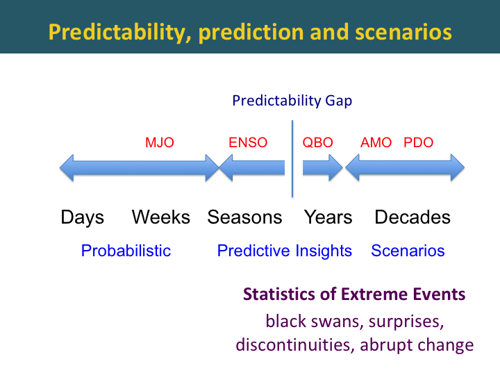
A predictability gap is seen around 1 year, where there is very little predictability.  At longer time scales some predictably is recovered, associated with longer-term climate regimes.  However at longer time horizons, predictions become increasingly uncertain.

Possible future scenarios can be enumerated but are not ranked, e.g. because of ambiguity.

A useful long range forecast keeps open the possibility of being wrong or being surprised, associated with abrupt changes or black swan events.   Anticipating abrupt changes or black swan events would be most valuable. 

The key forecasting challenge is is to extend the time horizon for meaningful probability forecasts, and to extend the time horizon for predictive insights of the likelihood of future events.

How can we extend these forecast horizons?

 

ECMWF ENSO prediction skill

Improvements to global climate models are helping extend the time horizon for meaningful probabilistic forecasts.

This slide compares El Nino Southern Oscillation forecasts from the latest version of the European model with the previous model version. The y-axis is the initialization month, and the x-axis represents the forecast time horizon in months. The colors represent the strength of the correlation between historical forecasts and observations.

The most notable feature of this diagram is the spring predictability barrier.  If you initialize a forecast in April, it will rapidly lose skill by July, and the correlation coefficient drops below 0.7 (which is reflected by the white region).   However, if the forecast is initialized in July, the forecast skill remains strong for 7 months and beyond.

The skill for the new version of the ECMWF forecast model is shown on the right, and we see substantial improvement.  While the color schemes are slightly different, you can see that the white region, indicating correlation below 0.7, is much smaller, indicating that the model performs much better during the springtime predictability barrier.

The improved skill in Version 5 is attributed to improvements to the ocean model and also to parameterizations of tropical convection.

 

Climate prediction: signal to noise problem

On timescales beyond a few weeks, the challenge is to identify the predictable components.  Predictable components include

• Any long-term trend
• Regimes and teleconnection patterns
• And any cyclical or seasonal effects

Once you identify and isolate the predictable components, you can ride the wave.

The challenge is to separate the predictable components from the ‘noise’.  These include

• Unpredictable chaotic components
• Random weather variability
• Model error

The biggest challenge is regime shifts, particularly when the shifts were triggered by random events.  You may recall that in 2015, it really looked like an El Nino wanted develop.   However, its development was thwarted by random but strong easterly wind outburst in the tropical Pacific.  This failed 2015 El Nino set the stage for the super El Nino of 2016.

 

Climate prediction: can we beat climatology?

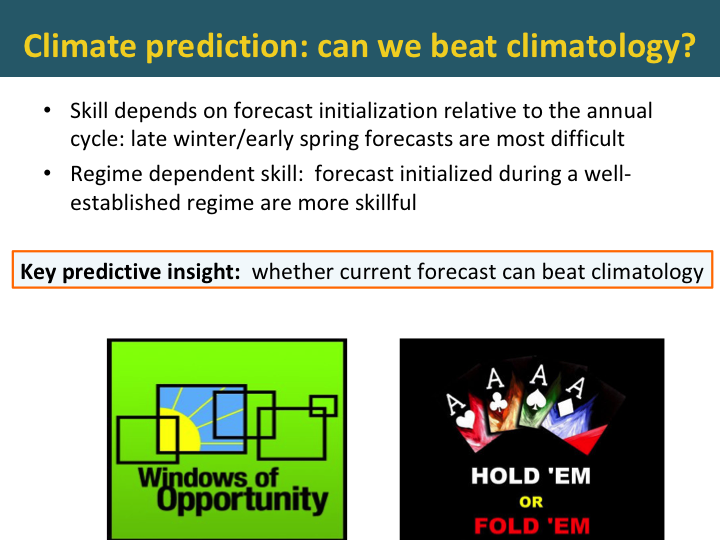
The big challenge in making a climate prediction is whether you can beat climatology. Forecast skill depends on several things.

When the forecast is initialized relative to the annual cycle is an important determinant of skill.  Also, a forecast initialized during a well-established regime, such as an El Nino, are more skillful.

One of the most important predictive insights that a forecaster can provide is whether the current forecast can beat climatology

The forecast windows of opportunityapproach identifies windows in time and space when expected forecast skill is higher than usual because of the presence of certain phases of large-scale circulation patterns.

I often use a ‘poker’ analogy when explaining this to energy traders – you need to know whether to ‘hold’ or ‘fold’. In forecasting terms, this is the difference between a forecast with high or low confidence.

 

Data-driven prediction methods

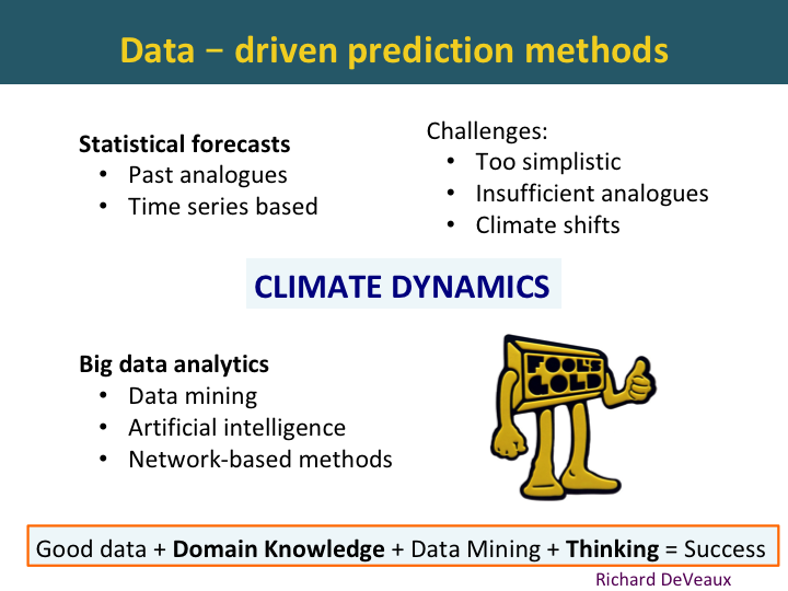
Statistical forecasts have been used for many decades before global climate models were developed, notably for Asian monsoon rainfall.  Traditional statistical forecasts have been time-series based or based on past analogues. While these methods do include insights from climate dynamics, they have proven to be too simplistic and there are an insufficient number of past analogues.

The biggest challenge for statistical forecasts is that they stop working when a regime shifts.  You may recall in 1995 when Bill Gray’s statistical hurricane forecast model stopped working, when the Atlantic circulation pattern shifted. A more recent example is use of October snow cover in Siberia as a predictor of wintertime temperatures, this one also stopped working once the climate regime shifted.

Currently, big data analytics is all the rage for weather and climate prediction.  IBM’s Watson is an example.  Mathematicians and statisticians are applying data mining and artificial intelligence techniques to weather and climate prediction.

Artificial intelligence guru Richard DeVeaux provides the following recipe for success:

Good data + Domain Knowledge + Data Mining + Thinking= Success

The limiting ingredients are domain knowledge andthinking.  Without a good knowledge of climate dynamics,  fools gold will be the fruit of any climate forecasts based on data mining.

 

Seasonal to interannual predictions: predictive insights –> probabilistic forecasts

The way forward in pushing the time horizon further for meaningful probabilistic forecasts is to integrate global climate model forecasts with insights from data driven forecast methods.

The problem with climate model forecasts is that they invariably revert to climatology after a few months.  The problem with data driven forecasts is that they lack space-time resolution.

These can be integrated by clustering the climate model ensemble members based on predictors from the data-driven forecasts.

Confidence assessment can be made based on the probability of regime shift.

 

Data-driven forecasts:  climate dynamics analysis

In data-driven approaches to climate prediction, it is essential to understand the range of climate regimes that can influence your forecast. These regimes indicate memory in the climate system.  The challenge is to identify the appropriate regimes, understand their impact on the target forecast variables, and to predict future shifts in these regimes.

CFAN’s analysis of climate dynamics includes consideration of these 5 time scales and their associated regimes, ranging from the annual cycle to multi-decadal time scales.

 

Circulation modes: sources of predictability

 Our data mining efforts have identified a number of new circulation regimes that are useful as predictors over a range of time scales. These include:

• North Atlantic ARC pattern
• Indo-Pacific-Atlantic pattern
• Northern and southern hemispheric stratospheric vortex anomalies
• Bi Polar patterns in the stratosphere
• NAOX:North Atlantic SLP/wind pattern
• Global patterns of North –South winds in upper troposphere/lower stratosphere

 

North Atlantic ARC pattern

An intriguing development is underway in the Atlantic. This figure shows sea surface temperature anomalies in the Atlantic for May.  You see an arc of cold blue temperature anomalies extending from the equatorial Atlantic, up the coast of Africa and then in an east-west band just south of Greenland and Iceland.  This pattern is referred to as the Atlantic ARC pattern.

 

North Atlantic ARC SST anomalies

A time series of sea surface temperature anomalies in the ARC region since 1880 shows that changes occur in sharp shifts, you can see shifts occurring in 1902, 1926, 1971, and 1995

On the bottom graph, you see that the ARC temperatures show a precipitous drop over the past few months.  Is this just a cool anomaly, similar to 2002? Or does this portend a shift to cool phase?

CFAN’s research has identified precursors to the shifts, we are actively assessing the current situation.

 

Atlantic AMO cool phase: impacts

A shift to the cool phase of the Atlantic Multidecadal Oscillation is expected to have profound impacts, based on past shifts:

• diminished Atlantic hurricane activity
• increased U.S. rainfall
• decreased rainfall over India and Sahel
• shift in north Atlantic fish stocks
• acceleration of sea level rise on NE U.S. coast

 

AMO impacts on Atlantic hurricanes

The Atlantic Multidecadal Oscillation has a substantial impact on Atlantic hurricanes.  The top figure shows the time series of the number of Major Hurricanes since 1920. The warm phases of the AMO are shaded in yellow.  You see substantially higher numbers of major hurricanes during the periods shaded in yellow

A similar effect of the AMO is seen on the Accumulated Cyclone Energy.

 

AMO impacts on U.S. landfalling hurricanes

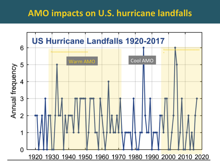
By contrast, you see that the warm versus cool phases of the AMO has little impact on the frequency of U.S. landfalling hurricanes.

 

AMO impacts on FL hurricanes

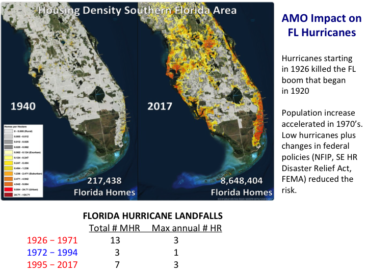
However, the phase of the Atlantic Multidecadal Oscillation has a huge impact on Florida. During the previous cold phase, no season had more than 1 Florida landfall, while during the warm phase there have been multiple years with as many as three landfalls. A major hurricane striking florida is more than twice as likely during the warm phase relative to the cool phase.

These variations in Florida landfalls associated with changes in the AMO have had a substantial impact on development in Florida.  The spate of hurricanes starting in 1926 0’ killed the economic boom that started in 1920.  Population and development accelerated in the 1970’s, aided by a period of low hurricane activity.

 

CFAN’s seasonal forecasts of Atlantic hurricanes

CFAN’s approach examines global and regional interactions among ocean, tropospheric and stratospheric circulations.  Precursor patterns are identified through data mining, interpreted in the context of climate dynamics analysis, and then subjected to statistical tests in hindcasts.

We consider three periods in our analysis, defined by current circulation regimes:

• The period since 1995, corresponding to the warm phase of the Atlantic Multidecadal Oscillation
• The period since 2002, defined by a 2001 shift in the North Pacific Ocean circulation patterns
• The period since 2008, characterized by a predominance of El Nino events, occurring every 3 years.

 

CFAN’s forecast for the 2018 atlantic hurricane season

Last week, we issued our third forecast for the 2018 Atlantic hurricane  season. We are predicting below normal activity, with an ACE value of 63 and 4 hurricanes.

The figure on the right shows hindcast verification for our June forecast model for the # of hurricanes.  The forecast is developed using historical data for 3 different periods, corresponding to the 3 regimes described earlier.

 

CFAN’s predictors for seasonal atlantic hurricane forecast

CFAN’s seasonal predictors are identified for each forecast using a data mining approach, with different predictors used for each lead time. The candidate predictors are then subjected to a climate dynamics analysis to verify that the predictors make sense from a mechanistic point of view.

The predictors that we use are predominantly related to atmospheric circulation patterns.  Note, our predictors differ substantially from other groups providing statistical forecasts, who rely primarily on sea surface temperature and sea level pressure predictors.

 

2017 seasonal forecast

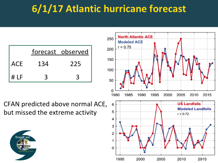
Here is the forecast we made a year ago for the 2017 Atlantic hurricane season. We predicted an active season with 3 U.S. landfalls.  We got the number of U.S. landfalls correct, but we substantially underestimated the Accumulated Cyclone Energy, or ACE.

From the perspective of the financial sector, the key issue is whether we will see another extremely active hurricane season and how that will translate into U.S. landfalls.

 

Atlantic hurricane forecast: worst case scenario

We conducted a data mining exercise to identify patterns that explained the extremely active seasons in 1995, 2004, 2005, 2017.  Our current forecast model does capture the extremes in 1995 and 2017, but not 2004 and 2005.

The only predictor that popped up for 2004/2005 is a pattern in the stratosphere near Antarctica.  At this point we have no idea whether this pattern could provide a plausible physically based predictor for Atlantic hurricane activity.  The disturbing thing tho, is that polar stratosphere predictors predict an extremely active 2018 season in contrast to the other predictors we are using.

So at this point we don’t know weather we have unearthed a diamond or fools gold.  In any event, this is a good example of both the promise and perils of data mining.