
Guest “Fracking A, Bubba,” by David Middleton
The Haynesville Shale (technically Haynesville/Bossier) in northeast Texas and northwest Louisiana is the third largest natural gas play, in terms of production rate and proved reserves, in these United States. Haynesville gas production set a record high in 2021 and will likely break that record this month.
APRIL 13, 2022
Haynesville natural gas production reached a record high in late 2021Dry natural gas production from the Haynesville shale play in northeastern Texas and northwestern Louisiana reached new highs in the second half of 2021, and production has remained relatively strong in early 2022. Haynesville natural gas production accounted for about 13% of all U.S. dry natural gas production in February 2022.
Haynesville is the third-largest shale gas-producing play in the United States. The Marcellus play in the Appalachian Basin (mainly in Pennsylvania, West Virginia, and Ohio) is the highest-producing shale gas play in the United States. During 2021, an average of 31.7 billion cubic feet per day (Bcf/d) of natural gas was produced from the Marcellus play. In the Permian play in Texas and New Mexico, production averaged 12.4 Bcf/d in 2021, making it the second-highest producing play. Altogether, the Marcellus, the Permian, and the Haynesville account for 52% of U.S. dry natural gas production.
Natural gas production in the Haynesville declined steadily from mid-2012 until 2016 due to its relatively higher cost to produce natural gas compared with other producing areas. At depths of 10,500 feet to 13,500 feet, wells in the Haynesville are deeper than in other plays, and drilling costs tend to be higher. By comparison, wells in the Marcellus in the Appalachian Basin are shallower—between 4,000 feet and 8,500 feet. Years of relatively low natural gas prices meant it was less economical to drill deeper wells. However, because natural gas prices have increased since mid-2020, producers have an incentive to increase the number of rigs in operation and use those rigs to drill deeper wells.
Producers tend to increase or decrease the number of drilling rigs in operation as natural gas prices fluctuate. The number of natural gas-directed rigs in the Haynesville has been rising steadily since the second half of 2020 and reached an average of 46 rigs in 2021, according to data from Baker Hughes. Since the beginning of 2022, producers have added 17 rigs in the Haynesville region. For the week ending April 8, there were 64 natural gas-directed rigs operating in the Haynesville, representing 45% of natural gas-directed rigs currently operating in the United States.
Pipeline takeaway capacity out of the Haynesville has also increased in recent years. The additional capacity allows producers to reach industrial demand centers and liquefied natural gas terminals on the U.S. Gulf Coast. The Enterprise Products Partners’ Gillis Lateral pipeline and the associated expansion of the Acadian Haynesville Extension entered into service in December 2021. Prior to that project, Enbridge Midcoast Energy’s CJ Express pipeline entered into service in April 2021. These projects added 1.3 Bcf/d of takeaway capacity in the Haynesville area, which is currently estimated to total 15.9 Bcf/d according to PointLogic.
Principal contributor: Katy Fleury
Tags: production/supply, natural gas, shale, Haynesville
Haynesville Features
Favorable Regulatory Environment
Haynesville pipeline takeaway expansion has not faced the same sort of political opposition as has plagued the Marcellus Shale. Texas has a very favorable regulatory environment, so favorable that only 33% of Texas Democrats support a ban on frac’ing.
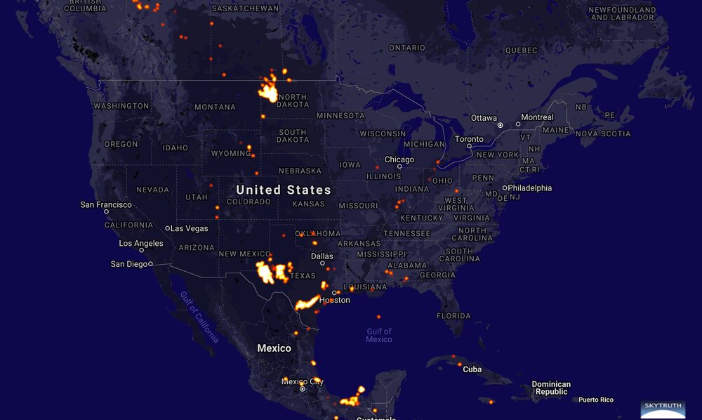
No Flaring Required
Being a nearly pure gas play, flaring is almost nonexistent in the Haynesville play.
Proved Reserves
At year-end 2020, the estimated proved gas reserves in the Haynesville stood at 44.8 trillion cubic feet (Tcf). If the Haynesville was a nation in Europe, it would rank second only to Norway (50.5 Tcf).
Note: the 1.9 Tcf decline in proved reserves from 2019-2020 is not due to there being less natural gas than previously thought. It’s due to low natural gas prices in 2020 (shamdemic effect). US oil and natural gas proved reserves declined in 2020. The decline was entirely due to price-driven revisions. Extensions and discoveries actually exceeded production by 2.7 Tcf.

Most increases in proved reserves are the result of field extensions, rather than new discoveries.
Discoveries include new fields, new reservoirs in previously discovered fields, and additional reserves that resulted from drilling and exploration in previously discovered reservoirs (extensions). Extensions typically make up the largest share of total discoveries. Beginning with the 2016 report, operators reported to us on Form EIA-23L their discoveries as a single, combined category—extensions and discoveries. Totals for that category are presented in one column on the data tables in this report.
U.S. Crude Oil and Natural Gas Proved Reserves, Year-end 2020 (EIA)
Extensions typically represent the conversion of probable reserves, possible reserves and contingent resources into proved reserves, based on well performance, infield drilling and other asset management efforts. Proved reserves only represent the volume of oil and/or gas with a >90% probability of being recovered.
Undiscovered Resource Potential
The most recent USGS assessment puts the undiscovered resource potential of the Haynesville shale (highlighted) at nearly 300 Tcf (~10 years of total US natural gas consumption).

Haynesville Formation, U.S. Gulf Coast, 2016. (USGS)
The Haynesville shale plays are the hachured and dotted areas on the map below…
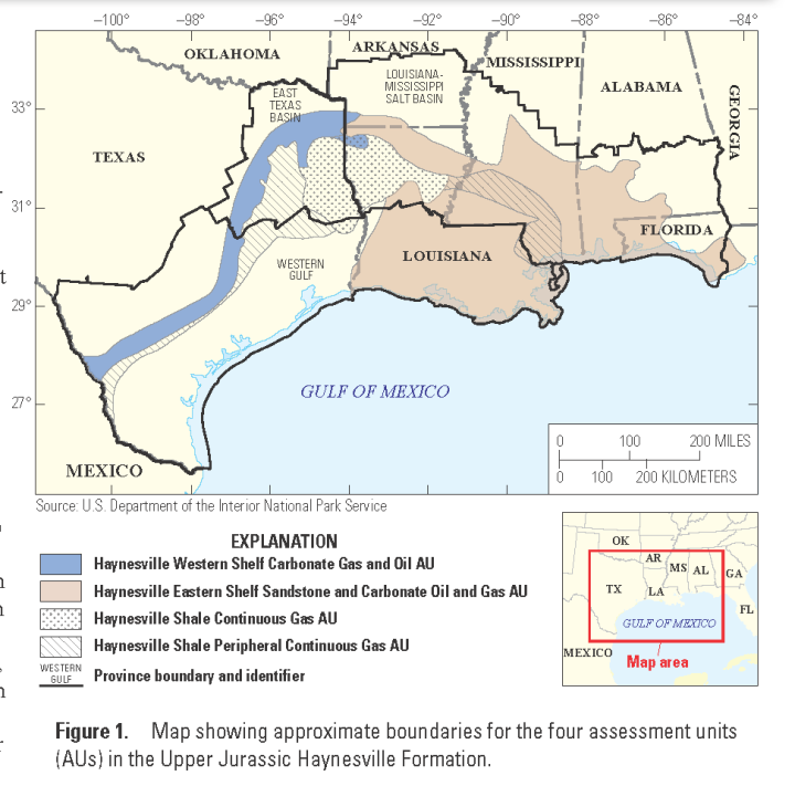
Haynesville Formation, U.S. Gulf Coast, 2016. (USGS)
The Many Benefits of Catastrophic Sea Level Rise
The Haynesville Shale, which has also been referred to as the “lower Bossier,” is the basinal equivalent
of the Cotton Valley Lime and pinnacle reef trend in East Texas that was deposited during the transgressive phase of SS2. These pinnacle reefs formed in response to the rising sea level as they were back-stepping onto Haynesville ramp carbonates; the carbonates were able to keep up with rising sea level until they were “drowned” by the fine-grained-sediment-dominated transgression. The top of the Haynesville Shale marks the maximum flooding surface as evidenced by maximum marine onlap on the shelf (e.g., Goldhammer, 1998). The Bossier shales (so-called “upper Bossier”) are characteristic of the highstand systems tract of SS2 reflecting a turn-around in sea level and increase in siliciclastic influence.
A marine transgression (catastrophic sea level rise), approximately 150 million years ago, led to the deposition of the Haynesville Shale, as well as the trapping mechanism for the Haynesville Shale and the stratigraphically equivalent Cotton Valley Lime pinnacle reef plays.
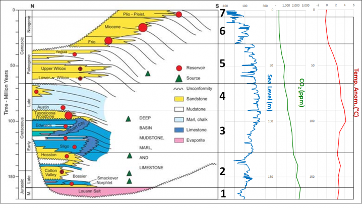
The hydrocarbons in the Haynesville Shale and Cotton Valley Lime were sourced from the Smackover and Haynesville Formations.
Mudstones within the Upper Jurassic Smackover and Haynesville Formations are sources of oil and gas
in both conventional (Montgomery, 1993a, 1993b; Mancini and others, 2006) and continuous reservoirs
(Hammes and others, 2011; Cicero and Steinhoff, 2013) throughout much of the assessment area.Assessment of Undiscovered Oil and Gas Resources in the Haynesville Formation, U.S. Gulf Coast, 2016. (USGS)
The Smackover Formation is probably the most prolific source rock in the Gulf Coast/Gulf of Mexico region. Depending on depositional environment, the Smackover is also a prolific oil & gas producer and the seal for the Norphlet Formation where it is productive. The Haynesville would be between the Bossier and Smackover Formations on the diagram below.
The next four displays are from Cicero & Steinhoff, 2013, depicting the sequence stratigraphy and depositional environments of the Haynesville and Bossier shales.


This is interpreted seismic profile A-A’, running from north (left) to south (right), just west of the Texas-Louisiana state line.

The following is a depositional environment (paleogeography) map of the Bossier Shale (~150 million years ago):
“You see the story yet?”
You see the story yet? It’s all pretty much here.
In a language you can’t yet understand, but it’s here.
A tale of upheaval and battles won and lost.
Gothic tales of sweeping change, peaceful times, and then great trauma again.
And it all connects to our little friend.
That’s what we are, we geologists.
Storytellers.
Interpreters, actually.
That’s what you gentlemen are going to become.
And how does this relate to the moon? From 240,000 miles away you have to give the most complete possible description of what you’re seeing.
Not just which rocks you plan to bring back but their context.
That and knowing which ones to pick up in the first place is what might separate you guys from those little robots.
You know, the ones some jaded souls think should have your job.
You see, you have to become our eyes and ears out there.
And for you to do that, you first have to learn the language of this little rock here.
–David Clennon as Dr. Leon (Lee) Silver, From the Earth to the Moon, Episode 10, Galileo Was Right, 1998
HBO’s 1998 From the Earth to the Moon miniseries was a sort of follow-on to the great movie Apollo 13… It’s a must see for space program fanatics. I particularly like this episode because my childhood interest in the space program led me toward the sciences and ultimately geology. Future Apollo 17 astronaut Harrison “Jack” Schmitt recruited his former field geology professor to train the Apollo 15 lunar module team and their backup crew how to become field geologists. It reminds me of why I love geology so much. I’ve also had the great honor of meeting Dr. Schmitt at the 2011 American Association of Petroleum Geologists convention in Houston. Shaking hands with someone who not only walked on the Moon, but also got to throw a rock hammer farther than any geologist ever has before or since, was pretty fracking cool… And so is geology!
References
Berner, R.A. and Z. Kothavala, 2001. GEOCARB III: A Revised Model of Atmospheric CO2 over Phanerozoic Time, American Journal of Science, v.301, pp.182-204, February 2001.
Cicero, Andrea D. and Ingo Steinhoff, 2013, Sequence stratigraphy and depositional environments of the Haynesville and Bossier Shales, East Texas and North Louisiana, in U. Hammes and J. Gale, eds., Geology of the Haynesville Gas Shale in East Texas and West Louisiana, U.S.A.: AAPG Memoir 105, p. 25–46.
Galloway, William. (2008). “Chapter 15 Depositional Evolution of the Gulf of Mexico Sedimentary Basin”. Volume 5: Ed. Andrew D. Miall, The Sedimentary Basins of the United States and Canada., ISBN: 978-0-444-50425-8, Elsevier B.V., pp. 505-549.
Galloway, William E., et al. “Gulf of Mexico.” GEO ExPro, 2009, https://ift.tt/YwgNqPR.
Hammes, Ursula and Ray Eastwood, Harry Rowe, Robert Reed. (2009). Addressing Conventional Parameters in Unconventional Shale-Gas Systems: Depositional Environment, Petrography, Geochemistry, and Petrophysics of the Haynesville Shale. 10.5724/gcs.09.29.0181.
Miller, Kenneth & Kominz, Michelle & V Browning, James & Wright, James & Mountain, Gregory & E Katz, Miriam & J Sugarman, Peter & Cramer, Benjamin & Christie-Blick, Nicholas & Pekar, S. (2005). “The Phanerozoic Record of Global Sea-Level Change”. Science (New York, N.Y.). 310. 1293-8. 10.1126/science.1116412.
Ramirez, Thaimar, James Klein, Ron Bonnie, James Howard. (2011). Comparative Study of Formation Evaluation Methods for Unconventional Shale Gas Reservoirs: Application to the Haynesville Shale (Texas). Society of Petroleum Engineers – SPE Americas Unconventional Gas Conference 2011, UGC 2011. 10.2118/144062-MS.
via Watts Up With That?
April 15, 2022 at 04:52PM
