April was the 32nd warmest in England this year in figures going back to 1884, based on Daily Max temperatures.
In reality, as the graph shows all to clearly, April weather is highly variable here, with average temperatures running anywhere between 9C and 17C. Although last month was closed to the 1991-2020 average, this does not tell the whole story.
As the CET daily chart illustrates, temperatures stayed within the “normal” band, not going below the 5% or above the 95% values. However, there was a preponderance of warmer than average weather – weather being the operative word.
A month ago, I published the charts below, showing that the highest temperature in March was not exceptional by any means. However the lowest temperature was relatively high by historical standards. In other words, the monthly average was higher normal not because of unusually warm weather, but because of the absence of unusually cold weather.
The emergence of the Isthmus of Panama, starting around 5Ma, due to uplift of the Caribbean plate was a major event in Earth’s recent climate history. It altered the depth of cyclic glaciation, which resulted in oceans being 138m deeper than the present level 23,000 years ago. This article looks at the cycles that drive the climate trends that create glaciation and interglacials. Chart 1 provides the reconstructed temperature history based on EPICA Dome C and the Spratt 800kyr sea level reconstruction over the past 800kyr.
Chart 1 also shows the top of the atmosphere (ToA) solar electro-magnetic radiation (EMR) for July at 15N (left hand scale). The basic frequency of the solar EMR is 23kyr corresponding to what is termed Earth’s axial precession cycle, which is modulated by eccentricity of the orbit around the sun and axial obliquity, Over the last 1Myr, eccentricity has exhibited a period of 89kyr and obliquity a period of 39kyr.
Fourier Transform of Temperature and Sea level Histories
Fourier transformation of time based data transforms the data from the time domain to the corresponding frequency domain to tease out the significant cyclic components in the data. Chart 2 displays the frequency components inherent in the change in sea level for the sea level shown in Chart 1.
There are three period peaks in the frequency domain. The two shorter periods, 23.3kyr and 39.4kyr align reasonably well with precession and obliquity cycles. The peak at 102.3kyr is a little longer than the period of eccentricity in the present era. It is noted here that the time interval for the sea level data is 1kyr with 512 data points so the resolution for longer periods is quite poor.
Chart 3 provides the frequency domain for the change in temperature for the temperature data displayed in Chart 1.
Again the periods for eccentricity and obliquity are clearly apparent. The longer period merges into a broad spectrum of lower relative amplitude.
It is worth noting here that when a higher frequency signal is being modulated by lower frequencies, the resultant signal will have side bands created by the modulation. Table 1 sets out the sidebands for a carrier of 23kyr being modulated by 39kyr and 89kyr.
The temperature data exhibits sideband periods of lower relative amplitude than the three dominant cycles and close to the expected periods for the sidebands.
Combining both the temperature and sea level data into a scatter plot as in Chart 4 is used to correlate the two variables.
The regression coefficient of 72% for the polynomial fit indicates good correlation. The best fit occurs when sea level lags temperature by 5kyr. This aspect is covered in more detail later. It is noted here that the assessed temperature range covers 14C.
Frequency Domain for Solar EMR Data
Given that orbital cycles are clearly apparent in the historical temperature and sea level records, it should be possible to gain insight into the process of glaciation by examining how ToA solar radiation varies across the Northern Hemisphere. Panel 1 provides a series of frequency domain transforms for the solar signal at nominated latitudes and time of year as well as certain combinations nominated in the chart title. A section of the time domain data is shown overlaying each chart. These charts are based on 1Mkyr of data at 500 year intervals.
The top panel shows the dominance of the precession cycle in solar EMR in July at 15N. Truncating this data as shown in the second panel brings out the lower frequency modulation. Then integrating the truncated data amplifies the lower frequency component as shown in the third chart.
The fourth chart in the panel looks to the frequency components in the solar EMR for December at 65N. Here the obliquity component dominates and the sidebands of the precession cycle are also evident. The bottom panel combines the July 15N and December 65N to produce obliquity and precession components of similar amplitude to those observed in the sea level and temperature histories.
This panel provides guidance on how the solar EMR from various northern latitudes can be combined to resemble the frequency components of historical data for climate change.
Detailed Observation of Termination of Interglacials
Having assessed that Earth’s orbit plays a significant role in glacial cycles it is useful to consider what circumstances applied during the termination of previous interglacials. A question pertinent to the present time.
The above analysis indicates that there is a combination of factors that give rise to glaciation. Further observation revealed that one possible combination is the July solar EMR at 15N being above a certain threshold to provide atmospheric moisture along with sufficient September EMR at 65N to sustain the atmospheric moisture while the land cools below freezing. The latter produces an enabling window as depicted in Chart 5.
The termination window can be envisaged as an essential advection component at high latitude where the July solar EMR at 15N is not sufficient alone to have enough moisture in the atmosphere but has to be supported by high moisture being sustained into September.
Panel 2 looks at eight previous interglacial terminations applying the notion of a termination window as shown in Chart 5 in combination with July solar EMR being above 443W/m^2. Temperature and moisture curves use the left hand scale in (m) and (C ) and the July solar above threshold, the right hand scale in (W/m^2).
In chart A of the panel, the window opens at the same time the solar is higher than the threshold and sea level begins to fall. In chart B, the sea level started to fall in year -696kyr but the window closed and the sea level rose despite the July solar at 15N being well above the threshold; essentially ice accumulation was advection limited. In Panel C, the window opened while the July solar was declining but still above the threshold enabling sea level to fall. Panel D has false starts while the window is open but the July solar is too low. Sea level began to fall as soon as the July solar exceeded the threshold.
In Panel E the July solar is low and similar to the present time but the sea level is almost 12m higher than present as well as the temperature being correspondingly higher. The window is open and there is a false start at -404kyr while the July solar is reducing but the solar does not fall below the threshold enabling the sea level to decline from -400kyr but then levels out until the July solar begins to increase at -395kyr.
The temperature generally remains high until accumulation begins and then drops faster to its minimum than the sea level to its cycle minimum. The temperature remains close to its minimum once the sea level is 40m below the zero datum while sea level descends further at each upswing of the July solar.
Chart 6 presents the same data as the charts in Panel 2 but for the present time with projections based on now rising July solar and the termination window being open. July solar EMR will be above the threshold within 2000 years. There will need to be a substantial increase in land ice extent before the sea level falls at the projected rate. The temperature forecast is based on the sea level correlation from Chart 2 and the sea level projection is based on the rising July solar as correlated to the circumstances after -395kyr in chart E of Panel 2. The termination that began 395ka had a false start soon after the termination window opened but then recovered before a second false start 400ka but sea level did decline to the zero datum before the July solar reached the threshold and the decent accelerated from 395ka. It is likely Greenland was able to increase ice extent over the 5,000 years from 400ka to 395ka despite the July solar being lower than the threshold.
An important observation with regard the end of glacial episodes is that sea level begins ascending when the July solar starts to increase from its minimum. The solar intensity can be well below the solar intensity needed to initiate glaciation. This implies that there is a limiting factor to the amount of ice the land can carry before glacier calving cools the ocean sufficiently to slow the water cycle and the rising sea level accelerates the calving and mobility of large icebergs that were grounded before the sea level started to rise.
Further Observations & Conclusions
In terms of geological time, modern glacial/interglacial cycles are very short but in terms of human lifespan they can be observed as trends. The axial precession cycle that drives the cycle of glaciation is the climate trend setter from human perspective. The changes are detectable over modern human lifespans. For example, 246kyr ago, the sea level increased by 24m in 1000 years or average of 24mm/year according to the sea level reconstruction. This is ten times the current trend. From 17ka to 7ka the sea level rose 101m or average of 10mm/yr for 10,000 years; four times the current trend. At the maximum of the last glacial period, the temperature was 9.8C cooler than the average of the last millennium. 407ka the surface temperate was estimated to be 2.5C above the average for the last millennium.. Over the last 800kyr, the estimated temperature has ranged over 14C.
At the depth of the last glacial period, the sea level was 138m below the present level. Taking the ocean surface area as3.6E14m^2, the amount of ice sitting on land then compared with now was 50,000Gt. The area of land north of 40N is 5.3E13 so a drop of 138m in sea level corresponds to an average increase in elevation of 937m of that land or a difference to sea level of 1075m compared with the present. The linear change in temperature with sea level equates to 72C/km, which is approximately ten times the average lapse rate and consistent with a combination of the ratio of sea level to difference in sea level and average ice level over land north of 40N as well as the obvious fact that it is not possible to get a block of ice much above 0C. At the depth of glaciation, the glacier calving would be having a significant impact on lowering ocean surface temperature and reducing atmospheric moisture.
There is no doubt that Earth’s orbital cycles dominate the climate trends. The combinations of solar EMR with selected months were based on some knowledge of the snow forming process over land, which is energy intensive as well as dependent on autumn and winter advection from ocean to land and lower land latitudes to higher land latitudes. July solar EMR at 15N is the most significant contribution to atmospheric water in the northern hemisphere. At the present time, the solar intensity at 15N is almost constant from May through to August and is more than sufficient to fuel the boreal summer Hadley Cells.
The existence of the strong obliquity signal in the data indicates that the solar intensity at high latitudes also plays a role. Snow accumulation is a balance between snowfall and snow melt but the melt also increases with rising July solar EMR. History demonstrates the rising snowfall eventually dominates when sea level is high and most northern land is ice free. It is also likely that the ice accumulates first on high ground and northern slopes then advances downward from the high ground as the average temperature reduces due to the increasing ice coverage. It is noteworthy that the interglacial termination window has been open for 7kyr while the July solar has been above the threshold but melt has continued to dominate apart from minor periods of accumulation in the past millennium. The July solar EMR is now just below the threshold required to initiate glaciation. The oceans of the NH now have a strong warming trend that is producing increased snow extent and new snowfall records are a common occurrence. So far only Greenland is showing an increase in permanent ice cover with some parallels to 395ka.
In terms of interglacial termination windows and July solar, the state of Earth’s climate now is similar to 400ka with Greenland fully covered in ice by then and temperature now similar to then. It is already apparent that Greenland is gaining ice extent per Chart 7 and the summit is gaining elevation. These trends should at least be sustained and will accelerate when the July solar exceeds the threshold.
Other early indicators of the interglacial termination are reduction in depth of permafrost thaw particularly northern slopes near the Arctic Ocean. For example, the thaw depth of permafrost on the northern slope of Mount Marmot in Canada was reducing to 2002 before the site became inactive. Other examples of permafrost thaw depth reducing are Inigok and Awuna, both in Alaska within 150km of the Arctic Ocean.
The last 7kyr has been a relatively benign period in Earth’s climate with minor excursions in sea level and surface temperature compared with what will be observed over the next 2000 years and beyond. There are already early indicators of the changes ahead.
Footnote
This article was prompted by a comment from Tim Gorman on my last article where I mentioned Fourier Analysis. He made the observation that few climate publications use signal analysis tools common in engineering.
Part 2 will be what I term Weather Maker because it will look at shorter term cycles including a proposal from Bob Weber regarding solar variability.
The Author
Richard Willoughby is a retired electrical engineer having worked in the Australian mining and mineral processing industry for 30 years with roles in large scale operations, corporate R&D and mine development. A further ten years was spent in the global insurance industry as an engineering risk consultant where he developed an enduring interest in natural catastrophes and changing climate.
This latest story is conclusive evidence that climate “science” has lost all scientific credibility, and is no more than politicised propaganda:
:
The summer of 2023 was the hottest for 2,000 years in the northern hemisphere, according to new Cambridge University analysis.
Humanity has not known hotter weather since the early days of the Roman Empire and the birth of Jesus Christ, the latest study shows.
Overall, last summer was 2.2°C hotter on land than the average temperatures for the years between 1AD and 1890AD, when the industrial revolution was in full swing, pumping huge amounts of climate warming greenhouse gas into the atmosphere.
It was also almost 4°C hotter than the coldest summer in 536AD – when an ash cloud from a volcanic eruption is thought to have caused temperatures to plunge.
‘When you look at the long sweep of history, you can see just how dramatic recent global warming is,’ said co-author Professor Ulf Büntgen, from Cambridge’s Department of Geography.
Reliable weather records produced by scientific instruments only date back to 1850 when the industrial revolution was getting under way.
But by analysing tree rings, scientists were able to calculate how hot summers have been by the growth of the tree ring and chemical composition of the wood.
Trees have narrower growth periods – creating narrower rings – during cold periods and wider rings during hot periods.
So they claim to know the exact temperature of the NH to hundredths of a degree for the last 2000 years just by using tree rings, something that we do not even know now.
And tree rings are pretty much useless as an indicator of temperature, because they can vary in width because of changes in precipitation, not to mention CO2.
But what we do know about the climate that far back strongly suggests it has been much warmer during that time.
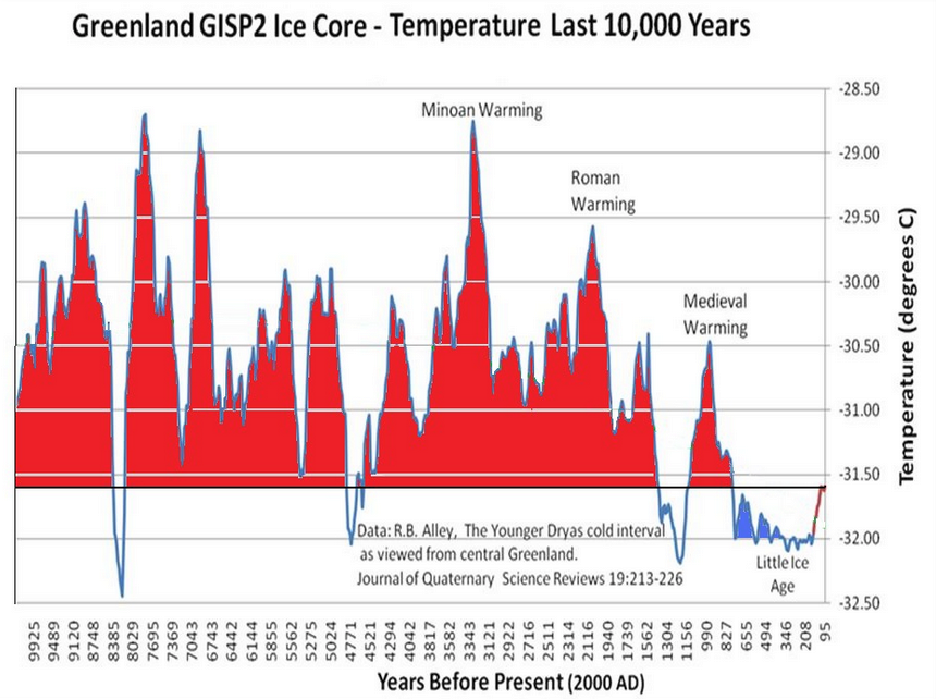
We know for instance that Greenland was considerably warmer than now during both Roman and Medieval times:
With Michigan Attorney General Dana Nessel filing the “climate” lawsuit that campaign supporter Michigan LCV had lobbied her to file against energy companies, and the UM law school faculty putting the shoulder to the wheel as well, GAO recalls the recently unearthed record of just how occupied Michigan’s government is with donor-financed “climate staff”.
First, recall Nessel’s embrace of taking in an activist lawyer provided by Michael Bloomberg to file this suit, just as Bloomberg-provided lawyers have filed numerous others for AGs from New York to Oregon:
And Michigan’s Public Service Commission asking for Bloomberg-provided “staff”, brokered by a renewable energy trade association “founded and funded” by Tom Steyer to push his agenda:
A Whitmer administration official hinted that Bloomberg’s group maybe might sprinkle a few more elsewhere:
To join the rest throughout the Whitmer administration, provided by “US Climate Alliance” (Hewlett Foundation, United Nations Foundation)(including the PSC Chair’s spouse):
Screenshot
It gets confusing which donor groups are to underwrite what state climate activism:
Asking them for three more each from USCA and the Rockefeller joint “Invest in Our Future”:
And, to top it off (so far as the public so far knows), telling Energy Foundation, come “invest in Michigan” government, with more bespoke climate “staff”:


