Author: Iowa Climate Science Education

Supreme Screw-up: Climate Fallacies Embraced by Canada’s Highest Court

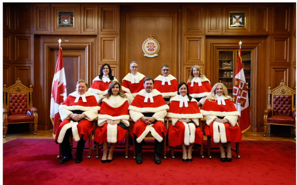
Canadian Supreme Court justices rendered an opionion regarding climate change that does not bear up under scrutiny.  Former government litigator Jack Wright exposes the errors in his C2C Journal article Supreme Screw-up: How Canada’s Highest Court Got Climate Change Wrong.  Excerpts in italics with my bolds and added images.

Many Canadians think of the Supreme Court as a wise and august body that can be trusted to give the final word on the country’s most important issues. But what happens when most of its justices get it wrong? Former government litigator Jack Wright delves into the court’s landmark ruling upholding the federal carbon tax and uncovers mistakes, shoddy reasoning and unfounded conclusions. In this exclusive legal analysis, Wright finds that the key climate-related contentions at the heart of the court’s decision were made with no evidence presented, no oral arguments and no cross-examination – and are flat wrong. Now being held up as binding judicial precedent by climate activists looking for ever-more restrictive regulations, the decision is proving to be not just flawed but dangerous.

The Supreme Court of Canada sits at the apex of the Canadian judicial ladder. But like any group of humans, the reasoning of its nine justices isn’t always right. What happens if the court’s reasons for decision include some mistakes and some confusing or inconsistent comments? Are all of Canada’s lower courts bound by these “precedents”? The short answer is no: a court’s decision is only precedent-setting for what it actually decided, and not concerning all of the detailed explanations for how the court got there. Still, erroneous reasoning at the top can create major problems as it often triggers unnecessary and harmful litigation that treats errors as binding precedents. That has proved to be the case with the errors in a crucial case that has profound economic, political and social implications affecting all Canadians.

Advocates for ever-increasing climate action have pounced on the decision in the case known as Reference re Greenhouse Gas Pollution Pricing Act, 2021 as precedent to justify further climate-related litigation, as if the courts or Parliament could stabilize the global climate. Such “lawfare”, as these kinds of tactics have come to be known, continues largely because of the non-binding comments in Greenhouse Gas. But the motivating claim – that these explanatory comments are binding precedents – is wrong.

They also misunderstand the special nature of a reference case.

In Canadian law a reference case is a submission by the federal or a provincial government to the courts asking for an advisory opinion on a major legal issue, usually the constitutionality of particular legislation. The opinion given by the Supreme Court is in the form of a judicial decision; strictly speaking, it is not legally binding, although no government has ever ignored such an opinion.

In Greenhouse Gas, the provinces of Ontario, Saskatchewan and Alberta sought the Supreme Court’s opinion on the constitutionality of the federal carbon tax, with all arguing that it is unconstitutional. In March 2021, a 7-2 majority upheld as constitutional Ottawa’s imposition of “backup” federal carbon pricing in any province which has no equivalent provincial measures. It did so based on the national concern doctrine (under the “peace, order and good government” clause in Canada’s Constitution).

In doing so, the majority unusually delved into the wisdom of climate and energy policy, which requires complicated scientific knowledge and resolving conflicting political priorities. The majority assumed – without any evidence – some crucial scientific facts about the causes and effects of climate change. There was no such evidence because a reference case is initiated at the appellate level and, unlike lower trial courts, appellate courts normally have no fact-finding function.

The majority made two important scientific assumptions. First, it assumed that climate change poses a threat to the survival of humanity. Second, it assumed that Canada’s climate is substantially controlled by Canada’s own emissions of greenhouse gases, chiefly carbon dioxide (CO2). Based on these assumptions, it would follow that Canada can avert the harms of climate change to Canadians by reducing Canadian COemissions through a carbon tax.

Suffice it to say that the high court’s two critical premises around which the whole reference case hinged were not proven material facts because there was no evidence before the Court. They were merely the untested assumptions of the seven justices. The first of these key assumptions is highly arguable; the second is outright fallacious. I will address the second of these assumptions first.

The Fantasy of a “Carbon Wall” Around Canada and its Provinces

The majority’s written decision, authored by Chief Justice Richard Wagner, contains a crucial assumption about the physics and chemistry of climate change. . . It held that severely harmful effects of emissions will mostly be caused by – and affect – people situated closest to the geographical origin of the emissions. This is a fallacy which I have termed the “Carbon Wall”.

The Carbon Wall fallacy leads to the error that the federal government can more easily control what the majority termed “grievous” interprovincial impacts caused by CO2 emissions from adjacent provinces. In essence, that government action can “wall off” the effects of greenhouse gas emissions around their area of origin. In fact, there is no CO2 “wall” around any country, nor can one ever be placed around a province by judicial finding or bureaucratic regulation. Unlike local pollutants, CO2 molecules emitted in the United States or China can flow over Canada and all around the planet, and vice-versa. Weather may be largely local, but climate is ultimately global, and so is the movement (and any climate effects) of CO2.

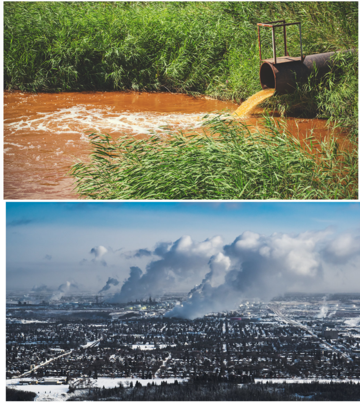
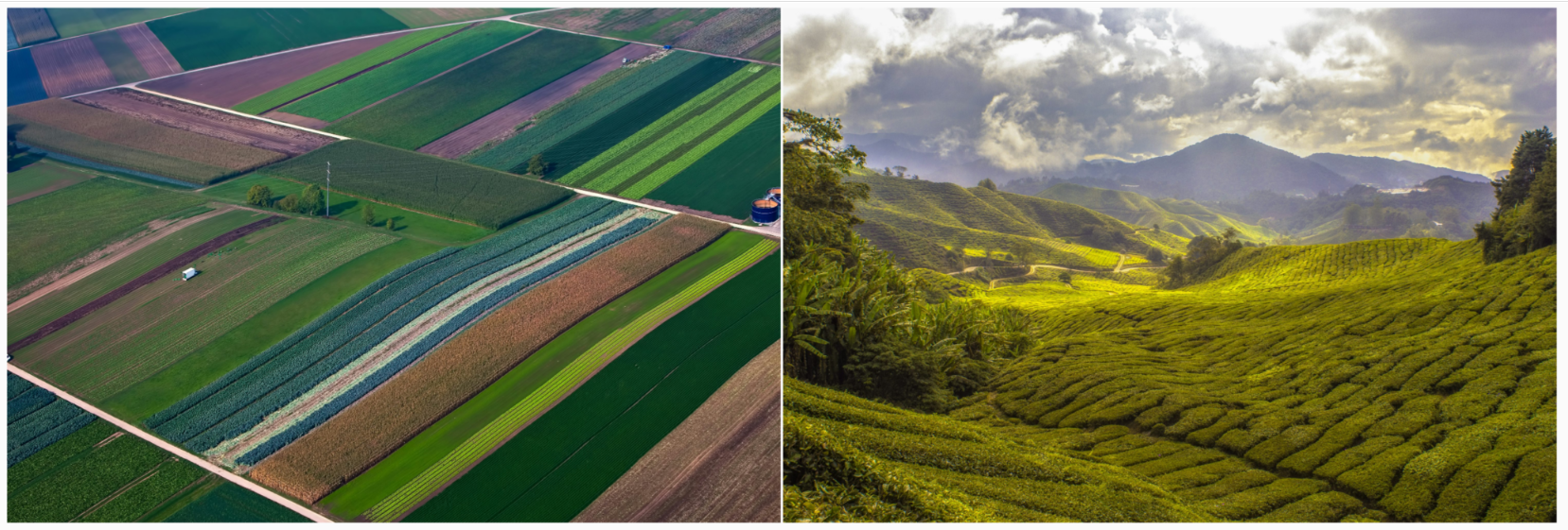
The “Carbon Wall” fallacy: The idea that local CO2 emissions cause local climate change is a common misunderstanding; Canada’s top justices accepted it, envisioning CO2 as akin to traditional pollution that might flow down rivers and cross provincial boundaries, and whose damage can therefore be locally controlled. (Sources of photos: (top) Shutterstock; (bottom) Daveography.ca, licensed under CC BY-NC-SA 2.0)

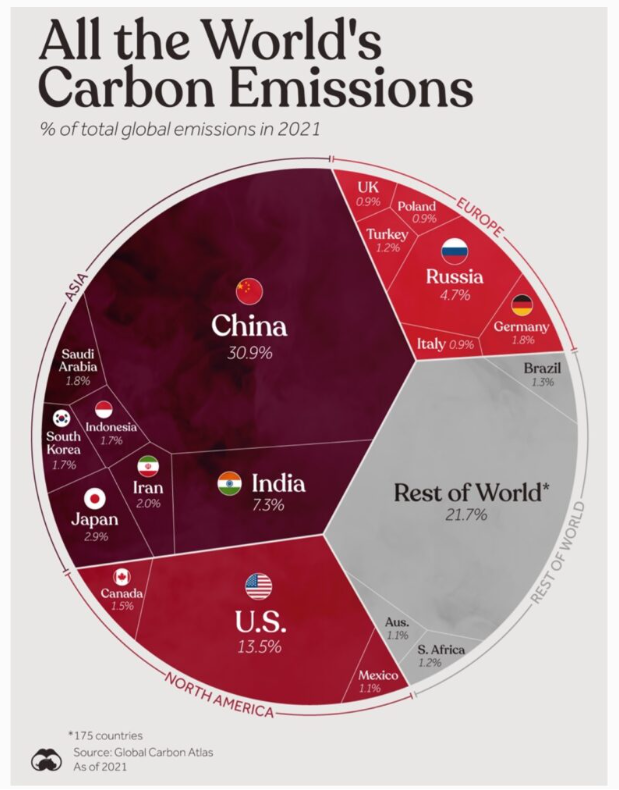
Thus, the majority assumed that climate change consists of CO2, following its emission, having a direct noxious climate impact upon geographically contiguous areas. We are not told, however, what particular form that harm takes, how it is caused or on what evidence it is based. But if Canada’s senior-most justices truly understood the basic mechanics of climate, they would have realized that virtually the entire impact of which they speak must come from outside the country, since Canada generates only 1.5 percent of global CO2 emissions, making each province only a tiny contributor to total global emissions.

Other Fallacious or Unsupported “Carbon Wall” Thinking

The majority also incorrectly suggested (para. 10) that, “The effects of climate change have been and will be particularly severe and devastating in Canada.” There is no evidence to support this assumption. While basic climatology holds that the Earth’s polar regions will warm more than lower latitudes, this is not unique to Canada. And rising levels of CO2 have also generated benefits through increasing agricultural productivity and forest and plant growth.

The good news: The Supreme Court said climate change would be “particularly severe and devastating in Canada”, an assumption for which there is no evidence; rising levels of atmospheric CO2 have actually led to a “greening” of the Earth, increasing agricultural productivity and forest and plant growth. (Source of photos: Pexels)

All that the Supreme Court’s ‘twice as fast’ alarm about Canadian warming shows is that Canadians live on land and not the ocean. The statement, while technically true, communicates nothing of significance. But it is highly misleading.

Canada is not bound in any meaningful way by the Paris Agreement, its contents should not influence decisions by Canadian courts, and the Supreme Court majority in Greenhouse Gas found nothing from the Paris Agreement that would be meaningfully precedential for those seeking to save themselves from ‘climate damage’.

The Assumption of an Existential Threat to Humanity

Climate change, Greenhouse Gas declares emphatically (para. 167), is “an existential challenge…a threat of the highest order to the country, and…[an] undisputed threat to the future of humanity [that] cannot be ignored.” It would seem to follow from this resounding pronouncement that the planet requires rapid decarbonization, with a massive and very costly diversion of resources to do so, and without regard to the cost trade-offs for other important human needs such food, housing and transportation or for such matters as safety and security.

Weighing such competing human needs is a political process, not a judicial judgment. Yet the Supreme Court’s assertions of catastrophe stand alone in mid-judgment, devoid of expert sources, of any investigation of facts, or of any reasoning from facts. This is unfortunate, because the court majority’s seemingly unqualified belief is anything but “undisputed”.

Many experts specifically dispute that humanity’s survival is at stake. Nobel Laureate William Nordhaus, the Yale University economist who is considered the “father” of the carbon tax, does so in his book The Climate Casino (page 134). Nor does the IPCC itself make such a claim.

“For most economic sectors, the impact of climate change will be small relative to the impacts of other drivers. Changes in population, age, income, technology, relative prices, lifestyle, regulation, governance, and many other aspects of socioeconomic development will have an impact on the supply and demand of economic goods and services that is large relative to the impact of climate change.” IPCC Report, Working Group 2, 2014

As Greenhouse Gas involved no evidentiary procedures, then what could have been the source of the Supreme Court’s ‘existential threat’ declaration? A search of the court files shows that this was assembled from an affidavit in Canada’s Record by a federal manager, John Moffet, an assistant deputy minister with Environment and Climate Change Canada.

Suffice it here to note that Canadian evidentiary rules do not allow for reliance upon a federal government manager’s affidavit for dispositive proof of an existential threat to an entire nation and indeed the whole planet. Moffet was neither disinterested in the dispute nor an expert on any aspect of climate science or any related scientific discipline that would qualify him as an independent expert witness.

The Unfolding Danger in the Supreme Court’s Climate Assumptions

There is no sense in parsing each of the assertions made by the majority in the Background, quite a few of which are highly questionable. But there is no existential threat inference to be drawn even if all are accepted. Climate change may be a serious problem, but it is only one among many other serious and resource-consuming human problems to be weighed and balanced.

If the Supreme Court of Canada chooses to evaluate complex climate policy in future (which the Court really lacks the institutional capacity to do), it should at least make arrangements for a full evidentiary record. For climate change, that would be enormous and would take months of hearings. A Royal Commission would be better placed to handle such a mission.

But judgments like Greenhouse Gas are wholly inadequate. It contains no true factual findings of an existential threat to humanity, or of a Carbon Wall around Canada, or of a possible Carbon Wall controllable by federal regulation around each of our provinces. There is no federal claim to be saving Canadians from interprovincial climate “pollution” and only a diffuse and very insignificant Canadian contribution to overall planetary climate change. Thus, the majority’s assumptions cannot serve as authority for the lower courts to adjudicate the cases that come before them under the guise of saving Canadians from climate change.

We cannot allow single-issue adherents (often wielding generous federal funding)
to repurpose our courts on pretextual bases and achieve goals
that they were denied through the ballot box.


via Science Matters

https://ift.tt/n0k1RqV

July 23, 2025 at 09:33AM

Forrest Mims: Top 10 Reasons to Keep Mauna Loa Observatory Open

As many of you know, the Mauna Loa Observatory (MLO) in Hawaii is slated for closure by the Trump Administration. Multiple reports indicate that the Trump administration’s proposed 2026 NOAA budget includes plans to defund the MLO. This would essentially lead to the closure of the observatory. The proposal also aims to shut down other atmospheric monitoring stations and eliminate a significant portion of climate research conducted by the National Oceanic and Atmospheric Administration (NOAA). 

In addition to being ground zero for global atmospheric CO2 measurements, it does many other things that are useful.

My friend, Forrest M. Mims III (One of the “50 best brains in science.” Discover magazine.) writes by email:

While I fully understand how the CO2 record begun there has led to the ongoing climate battle, MLO does far, far more than measure CO2. During my many stays at MLO (225 nights) I have never heard the long-time director, Darryl Kuniyuki, say a single word for, against, or about the CO2 record. He has far more responsibilities up there.

From my email to the Hilo Chamber of Commerce, which played a lead role in the establishment of MLO in the early 1950s, and which is stunned by the closure announcement:

The major factor in the closure of MLO is its pioneering role in measuring carbon dioxide since 1958 and the exaggerated publicity by climate change activists. This is unfortunate, for water vapor, not CO2, is the primary greenhouse gas. I have measured total column water vapor with instruments calibrated at MLO since 1990, and the trend is absolutely flat. (See A 30-Year Climatology (1990–2020) of Aerosol Optical Depth and Total Column Water Vapor and Ozone over Texas in: Bulletin of the American Meteorological Society Volume 103 Issue 1 (2022).

 Moreover, MLO does far more than measure CO2. For example:

 1.    MLO is the ultimate site to calibrate a wide range of instruments (including mine since 1993) that measure sunlight, ozone, water vapor, aerosols and various gases. Many organizations calibrate their instruments at MLO, including the Navy Research Lab, PREDE, Solar Light, MRI, NASA, PNNL, etc.

 2.    MLO data is invaluable for comparison with US, European, Japanese, and Indian satellite data, which drifts over time.

 3.  MLO’s remote location supports emergency communications during hurricanes, floods, earthquakes, and other emergency events. (I know this well, for I was staying overnight at MLO when a hurricane arrived.)

 4. MLO supports a wide variety of Federal and State government communications (Army, Navy, Civil Air Patrol, FAA, Hawaii Civil Defense, post office, etc.).

 5. MLO provides an important site for seismometers and tiltmeters that monitor potential volcanic activity of Mauna Loa.

 6. MLO’s helicopter landing zone is used for a variety of scientific studies and emergencies.

 7. MLO is a base of operation to rescue hikers on Mauna Loa.

 8. MLO has been used as an overnight rest site for military teams that search for and recover the remains of US military veterans lost in high-altitude airplane crashes. (I was staying there overnight when two such teams arrived.)

 9. MLO is an important site for visits by scientists and students studying a wide range of topics from alpine vegetation to rare alpine fauna. (I am among the few persons to see a Hawaiian hoary bat flying upslope while I was staying at MLO.)

10. MLO has become a vitally important site for my ongoing development and calibration of twilight photometers that measure the altitude of aerosols blowing from China to the US, high-altitude water vapor above the height of weather balloons, and both meteor smoke (85-90 km) and cosmic dust (100 km and above). (My twilight research began at MLO in 2013 and was compared with the MLO lidar.)


Discover more from Watts Up With That?

Subscribe to get the latest posts sent to your email.

via Watts Up With That?

https://ift.tt/q5hlHmD

July 23, 2025 at 08:03AM

The Reification of Averages – Part One. How the Met Office manipulates measurements.

Reification is defined as:

The act of treating something abstract, such as an idea, concept, or relationship as if it were a concrete, tangible thing, essentially turning something non-physical into something perceived as a concrete object or entity. This can occur in various contexts, from everyday language to social theory.” 

Although a rarely used word, its definition is something meteorology applies on a very regular basis. When you hear the weather forecaster announcing “that’s 10 degrees warmer than it should be for the time of year” you are being subjected to reification of a totally abstract, indeed usually completely non-existent, concept.

The headline image is taken from an essential reading short book written by Darell Huff in the 1950s that is possibly even more relevant in the 2020s than it was when written. It is now free to read online here

https://mronline.org/wp-content/uploads/2019/05/HowToLieWithStatistics.pdf

Many of the aspects covered by Huff relate very well to how the UK Met Office (and meteorology in general) portrays its data and how this is then “lapped up” by much of the media. I would like to expand upon Stephen Connolly’s excellent article on comparing temperatures past and present with special regard to how modern instrumentation, Stevenson screen siting, spurious maintenance standards, Victorian design and technology and instrumentation can readily be used to “achieve” preset end results and how such abstract concepts take on an almost reality life of their own.

This is my 300th post since restarting the Surface Stations Project 24/8/2024 and marks the beginning of summarising issues identified so far in my research. Further parts will follow, for now the averaging system.

Normal ” Averaging.

Take a sample of 10 adult humans, 9 are fully able but one has sadly had a leg amputated. Crude averaging of this sample could say the average number of legs is 1.9 per person i.e. 19 legs divided by 10 people. This could then be extended to claim 9 people were above average in respect of their number of legs and one was below average. Nobody was actually the “average”.

Obviously the above is a ridiculous example and such a dubious construct would never be used, or would it? In 1960s Britain there was a widely banded statistic that the average family had 2.4 children and that term almost passed into folklore with a TV sitcom spun off it. Even the Office of National Statistics recently referred to it. https://blog.ons.gov.uk/2019/08/02/whatever-happened-to-2-point-4-children/ This was a classic example of reification, a completely abstract and impossible figure (there is no such thing as “point four” of a child and never has been) was being taken as accepted fact. Social science analysis and even house design was being driven by this reified fictional notion.

To take this point a stage further imagine a sample of 24 people’s earned income. One person does not work and has zero earned income. Another is a reasonably high earner on £100,000 per annum, the remaining 22 all earn exactly £30,000 per annum each. What the “average” income actually is depends on which type of averaging system chosen. It is reasonable to assume most people would consider the “average” to be £30,000 per annum i.e. the mode or most common point. An arithmetic mean would derive 22 times £30,.000 = £660,000 + £100,000 + £0 divided by 24 = £31,667 so not that different to the mode. However, according to meteorological averaging the figure derived would actually be £50,000 – not even remotely close to any of the sample groups actual earnings. 23 people would be deemed below average income, only 1 above average. How does this work and why?

Meteorological Averaging.

This works to its own unique system. Daily average (“mean”) temperature is derived from adding together the daily minimum to the daily maximum and then dividing by 2 . This demonstrates how the “average” income of £50,000 in the above example was derived. This is despite the fact that it is routine for the Met Office (and even the public) to have access to 24 separate hourly readings per day, every day of the year – in fact most Met Office automatic weather stations produce 1,440 readings per day on a minute by minute basis.

An example of this minute by minute “extremes effect” were the details revealed behind a daily national high at Cavendish. In this case the “high” lasted for just 1 minute and was bizarrely quoted to the 5th decimal place from equipment only calibrated to the first decimal place. As former Met Office manager, John Maynard commented that this “just showed the stupidity of the observer.” Similar one minute readings established the crossing of a somehow “scary” threshold at Wiggonholt.

This Meteorological averaging principle emphasises extremes rather than represents the norm and consequently regularly produces bizarre and nonsensical results. As I reported in the comparison of the months of May 2024 with May 2025 , the former dank, damp and dismal May 2024 was deemed considerably “hotter” than the record sunshine, dry and warmer conditions of May 2025. Through the reification of this nonsense by the argument from authority of the Met Office, this somehow managed to make both months indicative of an impending doom.

Deriving data from solely extreme inputs can produce even more absurd outcomes. In the 24 person income scenario above, if that one person formerly without income were to start earning at exactly the same rate as the 22 majority (i.e. £30,000 per annum), then meteorological style averaging would suddenly make the average income ( now £30,000 minimum + £100,000 maximum ÷ 2) = £65,000. All those earning £30,000 have just fallen an even longer way further behind the “average” income instantaneously!

It is worth bearing in mind that, whilst it is standard practise in statistics to eliminate extremes or “outliers” (typically the top and bottom 5 or 10%) in order to avoid skewing averages, meteorologists solely use such normally excluded aspects. Small marginal changes can cause almost seismic variations.

History

This clearly outdated averaging system derived from the earliest attempts to standardise temperature recording. At one time knowing what the highest or lowest temperature of the day in the open air actually was would have required physically viewing the thermometer continuously – unsurprisingly that never happened. Initially readings were taken at set times per day but even that presented difficulties in that time itself was not standardised in the UK until the railway era. Prior to this change “local time” operated largely by the parish church clock and approximations of solar time hence no simultaneity of readings could be guaranteed.

GMT was ultimately adopted across Great Britain by the Railway Clearing House in December 1847. It officially became ‘Railway Time’.

By the mid-1850s, almost all public clocks in Britain were set to Greenwich Mean Time and it finally became Britain’s legal standard time in 1880.

Realistically it was not until the advent of Six’s maximum/minimum thermometer in 1780 that any passably reliable direct readings could be taken though even these were initially subject to dubious calibration . This thermometer gave fixed points of the extremes that could be read at approximately the same time each day without corruption if early enough in the morning. It must be noted that even this system works on assumptions. The maximum reading shown at 9:00 is assumed to be from the day before, whilst the minimum is attributed to the day of the reading. This often is not the case for example when a warm front displaces a cold one overnight or vice versa. A very cold day may be followed by a warmer night and the readings attributions can be the wrong way around.

It was not until Rutherford considerably improved the Six design in 1790 that readings became more accurate but the day attribution issue still remains to this date at manual stations despite the fact that everyone of them has an electronic Platinum Resistance Thermometers (PRT) for at least the maximum readings with a continuous readout held in its memory. {n.b. Liquid in Glass Thermometers (LIGT) are usually retained for minimum readings.}

This production of just 2 readings per day and only of the extremes is the origin of this unrepresentative averaging system – and thence, unlike any other branch of science, this seems to have been set in stone and apparently CANNOT (or rather will not) be changed.

Despite all the options that have been available since with improved metrology , the Met Office, and other meteorological institutions, have maintained this averaging system derived almost from antiquity. Those temperatures forecasters claims to be above or below what “it should be”/ “ought to be” /”what we would expect for the time of year” et alia are in fact simply the reifications of a terribly bad system and in reality are quite “mean-ingless”.

Problems caused by this system.

Authors Anthony Woodward and Robert Penn produced the delightfully interesting book “The Wrong kind Of Snow” which covers weather extremes for every day of the year together with interesting and entertaining associated weather facts. For most days of the year the book highlights the highest and lowest ever recorded temperatures which reveals the remarkably wide range of UK weather from year to year.

Whilst it might be assumed that extremes would be geographically driven they are in fact anything but. The overall maximum annual temperature differential according to the Met Office over recent times runs from minus 27.2 °C to 40.3 °C making a 67.5 °C range. Surprisingly even places close together can display a very large range

– On 10/3/1929 a temperature of 21.3 °C was recorded at Roade (Northants) whilst on the same day just 2 years later and under 40 miles away Rickmansworth shivered at minus 15 °C…….a 36.3 °C a largely only temporal differential.

– The notably mild south east England climate of Kent has recorded the low temperature of minus 21.3°C on a 30th of January whilst the same day in a different year the high was recorded as plus 15.5 °C. in north east Scotland…….. a 36.8°C both temporal and geographic differential.

What the above figures demonstrate is that there is no specific  temperature for any time of year or location but rather a very large potential range. Claiming any “should be/ought to be” for the time of year is a nonsense derived from the reification of an absurd averaging system resolving down extremes to unrepresentative “daily means”.

The current spate of Met Office “gaslighting” the UK public into comparing current summers to the exceptional summer of 1976 cannot be supported by the hard numbers of high temperatures exceeding thresholds. In lieu of the reality the Met Office resorts to its statistical misrepresentation tool of daily mean.

In 1976 there were  “16 consecutive days over 30 °C (86 °F) from 23 June to 8 July” far in excess of any subsequent summer heatwaves. However, in also being towards the end of a long term drought (which had started at the end of summer 1975) the weather also displayed desert-like (radiation frosts) daily temperature ranges to colder overnight temperatures. There were exceptionally rare “black frost” events recorded in southern England from the 28th to the 31st July. This aridity effect lowered the minima recorded and thence meteorological averaging took over to distort the reality of continuous very hot days, – archetypical “How to Lie with Statistics”

System Summary.

What is shown with this meteorological averaging system is that,

1. It is controlled by extremes regardless of how brief they may actually be. Just 2 separate 1 minute readings out of 1,440 can set the mean daily temperature.

2. It is outdated, only established by historic shortcomings and is failing to utilise the benefits of technological improvements.

3. It produces fixed headline numbers for reification.

4. Most importantly for some – it could easily be “played” or manipulated.

Playing the system. ……to be continued.

via Tallbloke’s Talkshop

https://ift.tt/nKH4l5w

July 23, 2025 at 06:33AM

VCEA could cause Dominion’s average customer to pay over $40,000 for batteries

The Virginia Clean Economy Act (VCEA) mandates that Dominion Energy, the state’s big electric utility, rapidly shift its power generation to wind and solar.

via CFACT

https://ift.tt/B1j2ZNs

July 23, 2025 at 05:06AM