News Brief by Kip Hansen — 16 January 2024 — 1100 words/5 mins
Antarctic ice melt has been an ongoing scientific controversy for more than a decade. Oddly, the warring parties are all at the same U.S. Federal Agency. The war, which involved salvos of papers between the NASA’s GRACE Ice Mass team and H. Jay Zwally and his team.
Here’s the background:
The current NASA Vital Signs of the Planet web page [NASA’s climate crisis propaganda section] for Ice Sheets carries this message boldly across the top one third of the page:
Here is today’s Vital Signs Antarctic Ice Sheets graphic:
It is important to remember that both the NASA’s GRACE Ice Mass team and Zwally et al. use the same data sets to determine their estimates of losses and gains. The differing results are then an indication of the different approaches to interpretation of that data, which may include biases.
NASA’s climate.gov doesn’t quite agree with Zwally et al. yet. But the Vital Signs graphic is for “Antarctic Ice Mass in Gts” . . . and that total ice mass has been level since turn of the century, with a lot of variation.
Compare Zwally’s 2021 estimate of -12 GT a year with the GRACE figure of -137 GT a year (in the two panel image, on the right). Zwally’s runs through the end of 2016.
Don’t think for a moment that Jay Zwally is some kook on the shady fringes of NASA – he is one of their top flight scientists and led the 2003 ICESat mission. He presented one of NASA’s famed MANIAC talks in 2019. And he has firmly stated that his Antarctic Ice Mass work is not a repudiation of climate science—it is just solid evidence that Antarctic Ice Mass is not plummeting as the Climate Crisis Team claims. (One might rightly ask why, then, don’t the creators of the Vital Signs Ice Sheets page present his results alongside of those of the GRACE team.)
So what’s the news?
The news is that some clever scientists — Collin M. Schohn, Neal R. Iverson, Lucas K. Zoe , Jacob R. Fowler, and Natasha Morgan-Witts — had decided that instead of blindly following the long-standing formulas for glacier ice flow, maybe they ought to find out, using real experiments, if those formulas actually reflect what happens in the physical universe where glaciers, ice under pressure, are flowing and melting. It took them ten years.
Disclosure: I am not a glaciologist. I know next to nothing about the physics of ice melting under pressure. Therefore, I report only what SciTechDaily says.
“New research shows temperate glacier ice flows more steadily than previously thought, leading to lower projections of sea-level rise.
Neal Iverson started with two lessons in ice physics when asked to describe a research paper about glacier ice flow that has just been published by the journal Science.
That temperate ice is like an ice cube left on a kitchen counter, with meltwater pooling between the ice and the countertop, he said. Temperate ice has been difficult to study and characterize.
Second, other parts of glaciers have cold, hard ice, like an ice cube still in the freezer. This is the kind of ice that has typically been studied and used as the basis of glacier flow models and forecasts.
The new research paper deals with the former, said Iverson, a paper co-author and project supervisor.”
The press release is about Iverson’s new paperLinear-viscous flow of temperate ice(Schohn et al. 2025). (paywalled and too new for my usual paywall-work-arounds).
“The paper describes lab experiments and the resulting data that suggest a standard value within the “empirical foundation of glacier flow modeling” – an equation known as Glen’s flow law, named after the late John W. Glen, a British ice physicist – should be changed for temperate ice. …. The new value when used in the flow law “will tend to predict increases in flow velocity that are much smaller in response to increased stresses caused by ice sheet shrinkage as the climate warms,” Iverson said. That would mean models will show less glacier flow into oceans and project less sea-level rise.”
How much less? Can’t read the paper, so I don’t know. [If anyone has access to the paper here, I’d love a copy].
But here is Iverson’s sketch of the experimental equipment which was all contained in a temperature-controlled freezer:
The press release further states:
“Resetting n to 1.0
Glen’s flow law is written as: ε ̇ = Aτn.
The equation relates the stress on ice, τ, to its rate of deformation, ε ̇, where A is a constant for a particular ice temperature. Results of the new experiments show that the value of the stress exponent, n, is 1.0 rather than the usually assigned value of 3 or 4.
The authors wrote, “For generations, based on Glen’s original experiments and many subsequent experiments mostly on cold ice (-2 degrees C and colder), the value of the stress exponent n in models has been taken to be 3.0.” (They also wrote that other studies of the “cold ice of ice sheets” have placed n higher yet, at 4.0.)”
Most of us might want to check the Wiki for an explanation of Glen’s Flow Law. The key is that the exponent n is just that, an exponent and not a mere multiplier. Thus, the call to re-set that exponent to “1” makes a rather huge difference.
The Bottom Line:
New research shows temperate glacier ice flows more steadily, linearly and not exponentially, contrary to our previous understanding, and this leads to far lower projections of future sea-level rise due to any glacier melt in Greenland and Antarctica.
# # # # #
Author’ Comment:
We have to admire a group that spends ten years, working through all the failures and development, to discover something closer to the real-world truth about something as hard to measure as “glacier ice flow” – the flow of ice under tremendous pressures – and the melting that takes place.
Hopefully, we will see the findings translated into better, more reasonable and less hysterical projections of future sea level rise that might result from the melting of the glacier ice of Greenland and Antarctica.
Comments meant for me should begin with “Kip—“ or some such.
I can be reached by email at my first name at the domain i4.net.
Thanks for reading.
# # # # #
Discover more from Watts Up With That?
Subscribe to get the latest posts sent to your email.
The Cloud Reduction Global Warming, CRGW, theory is a cascading natural process that only since about 1970 has become significant in Climate Change. The basic elements of CRGW theory have been around forever, it is the size (% of the earth affected) that has increased to the point that this natural process can be seen. The CRGW theory starts on land with the concept of a Special Parcel, SP, that has been changed from its virgin state such that less water is evaporated than the original virgin land. (SP examples: UHIs, forest to crop, or surface mining) The lower water evaporation (as indicated by lower surface air specific humidity, SH) creates higher temp and lower relative humid, RH, than the original land. How much a SP has changed the evaporation is not known since the original evaporation is not known, but if the land surrounding the SP is unchanged it can be used as a reference (the zero) for how much the SP has changed. The changed vs virgin land difference in SH remains relatively constant as the size of the SP increases with time. The SP’s lower humidity hotter air rises in a plume about 2 to 4 time larger than the land area it came from to cloud level: thus, amplifying the cloud level effect. The cloud cover is related to the Vapor Pressure Deficit, VPD, (the difference between the saturated water vapor pressure and the actual water vapor pressure). Higher VPD less clouds. The less clouds more Sun (lower global albedo). More Sun more atmospheric enthalpy, higher temperatures, and more evaporation of water (SH rising). This cascading series of natural events increase with the size of the earth’s total SPs. Simply put: if less water is put into the atmosphere from land (relative to what was evaporated previously) the global cloud fraction will decrease, and it will get HOTter.
The atmosphere fingerprint supports the CRGW theory: Since 1970 temperatures, specific humidity, enthalpy, and VPD have been rising while relative humidity and cloud cover have been declining. The lower evapotranspiration, ET, (proportional to SH) in over 1500 cities has been confirmed by Mazroonei et al (8). The existence of Urban Heat Island plumes has been modeled and weather balloons have confirmed their existence.
Reasonable estimates of global SP ET (or SH) change in a mathematical models suggest that CRGW could be a significant contributor to global warming and is reversable.
Introduction
This essay is intended to be a summary of all 7 previous essays (1),(2),(3),(4),(5),(6),(7) with the theme of CO2 is innocent, but Clouds are Guilty (thanks WUWT). To the reviewers of previous essays thanks for your suggestions and comments. I hope this essay will answer some of your comments.
In this essay ET change and SH change are used interchangeably. Evapotranspiration, ET, is defined as the total water flux evaporated into the atmosphere from surface Evaporation and plant Transpiration. Specific humidity, SH is the concentration of water in air. On an annual basis ET is proportional to surface SH. CRGW theory uses %ET change = %SH change. Change not the actual value.
Prior to about 1970 climate scientist assumed that the annual cloud cover and reflectivity of short-wave radiation of the earth were relativity constant, because there was no data to say otherwise (13). With the advent of satellite data that is changing. The “urban heat island effect”, UHI, was known but alone was too small to be a significant climate change variable. In this essay the UHI’s possible amplifying relationship to cloud reduction and climate change is presented. It is also suggested that other land changes could have similar UHI climate change properties.
CO2 is innocent
The main points of the innocents of CO2 are:
In the lower atmosphere CO2 is a greenhouse gas that absorbs long wave, LW, radiation and heats the atmosphere. The Beer-Lamber law says that this absorption is a function of distance and concentration (of CO2). At 400 ppm, CO2 is saturated in the lover atmosphere. Saturation means that more CO2 will not change the LW absorption in the lower atmosphere. The IPCC agrees. . See (1) and (2) for more information.
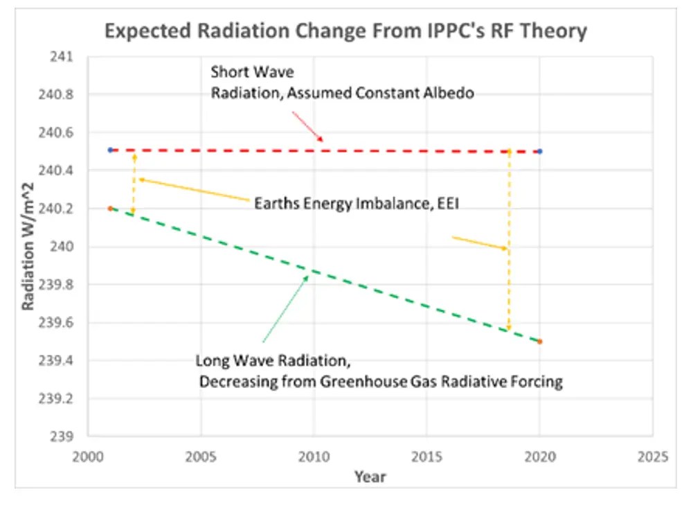
The IPCC’s current theory (radiative forcing, RF) is that in the upper atmosphere CO2 via Planck’s Law and Kirchhoff’s Law will absorb long wave radiation and reflect heat back to the lower atmosphere. To prove this theory NASA put the CERES satellite up to measure the radiation related to this theory. RF theory should show relatively constant short wave, SW, radiation out and decreasing long wave, LW, radiation out with time See Figure 1. Twenty years of CERES data analyzed by Dübal et al (15)and Loeb et al (16) show SW out decreasing and LW out radiation increasing over the 20 years, contrary to RF theory, see Figure 2. Their papers also indicated there may be some evidence of RF but clouds were the main source of SW and LW change over the 20 years.
Figure 1. Expected Radiative Forcing plotFigure 2. Dubal et al (15) CERES data
Decreasing relative humidity, RH, with time does not fit the RF theory.
Decrease in low altitude clouds and no change to high altitude clouds does not fit the RF theory. RF theory would support decreasing all altitude clouds
Another theory is needed to explain the CERES data and the atmospheric observations. CRGW theory does that.
CRGW Theory – Cascading Natural Steps.
The Special Parcel, SP
Clausius–Clapeyron law describes the atmospheric behavior in a special parcel, SP: as the SH decreases the temperature increases at a constant enthalpy, see Figure 3. As enthalpy increases this relationship increases. The density decreases as the temperature increases, the decrease in SH has little effect on the density change, see Figure 4.
Figure 3. ET (or SH) Change vs TemperatureFigure 4. ET (or SH) Change vs Density
In a SP the SH change is not known (invisible) because the starting SH is lost to time, but can be relative to surrounding virgin land. Clausius–Clapeyron laws apply to all SPs: urban UHIs, rural structures, forest to crop, surface mining, etc. Prior to 1970 the total area of all these SPs was not large enough to have much of an impact on climate change. All these SPs are sources of ET change (increase of decrease) vs what was there before the SP.
A wide range of ET from UHIs was verified by Mazrooei et al. (2021) (8) and Lu Hao et al. (2021) (9) with a creative method from satellite data. Their data shows SPs in arid environments can have positive ETs and SPs in wet environments have negative ETs, showing a ET range of +10% to -50%. With a -12% ET change globally. Mazrooei et al.’s work proves that the (invisible) starting step of the CRGW theory is real, significant, and negative. See (7) for more information.
Vapor Pressure Deficit, VPD and Clouds
From the SPs temperature and SH the saturation vapor pressure, Psw, and the actual water vapor pressure, Pw, can be calculated. The difference between these is the Vapor Pressure Deficit, VPD, and is a measure of the probability of condensation of water to clouds, fog, or rain. The lower the VPD the higher the probability of cloud formation. The VPD has been increasing over time and as expected clouds have been decreasing. This correlation, see Figure 5, is not that good, probability due to the fact that all clouds are not the same. Cloud cover includes dark rain clouds, non-rain clouds, high clouds, low clouds, and partly cloudy all these cloud types count in the cloud fraction but have a different correlation to VPD. CERES data (for 20 years) shows that cloud SW radiation reflectivity is a better correlation to the surface VPD, see (3) pie charts 3 and 4. A higher VPD vs cloud cover slope will decrease the cloud cover and thus the global temperature. See (5) for more information.
Figure 5. Global Cloud Cover (fraction) vs VPD. Figure 6. VPD vs global Enthalpy
The increase in SW radiation from the reduced cloud cover is absorbed by the earth to heat the land, oceans, and atmosphere as measured by the enthalpy. The En for the atmospheres can be calculated from the atmospheric (surface) temperature and SH and has increased with time. As expected En and VPD are correlated, see Figure 6. This slope of Figure 6 will be used in a mathematical model.
The increase in SW radiation is absorbed by water and evaporates water (mainly from the oceans). On land plant transportation is the main source of water to the atmosphere. The En vs SH correlation is good, see Figure 7. The slope of Figure 7 will be used in a mathematical model
Figure 7. Specific humidity vs Enthalpy
SPs that produce lower density air (hot air) tend to produce a plume. These plumes amplify the VPD correlation to cloud cover. Modeling has shown UHI plumes can be 2 to 4 time the area of the UHI they came from.
Data from weather balloons “Soundings” suggest that a plume of higher VPD air is created over cloud free UHI’s and can be 1 to 4 time greater than the area of the UHI. The plume is created by the lower density of the hot-lower humidity air (lower ET) rising from the UHI and forcing turbulence (mixing) with the much low humidity air in the upper atmosphere.
“Soundings” data show the VPD decreasing as the altitude increases. If the VPD nears zero clouds may form, see Figure 8. Higher surface VPD increases the probability that the rising air will miss zero and stay clear sky. Bigger plumes increase the area of no clouds. Lower SP air density from lower ET (higher temperature, Figure 2) may cause bigger plumes. See (6) for more information.
Figure 8. VPD vs altitude from a SP.
Figure 8. VPD vs altitude from a SP.
How much of the Earth is changed
Size matters, if the area of all the SPs on land is less than 2% the CRGW theory is insignificant in climate change; but if the SP area is around 10% the CRGW theory could account for most of the observed climate change. Table 1 shows how the area of several SP categories may have changed over the years. (Table 1 is a guess based on several internet sources.) The increase in area from the 1970s to the present suggest the very little CRGW significance in 1970 to significant in 2020.
Table 1. Possible area of Special Parcels on earth since 1860.
Put it all together mathematically
I created an Excel model linked here, using proven Clausius–Clapeyron related psychometrics equations and the correlations in Figures 5, 6, and 7 was developed with inputs of total earth area of SPs, Table 1, and the average ET (SH) change. See (4) for psychometric equations used and more information.
Verbal description of the model:
Pick a starting point global annual temperature (T) and specific humidity (SH) from on-line global data (11) and calculate the global Enthalpy and VPD. (example for 1975: T=14.01 ‘C and SH= 7.59 g/kg(da) calculated En=33.37 kJ/kg(da) and VPD = 3.82hP/kg(da))
Input an average change in SH to the sum-total of all the SPs on land. (example -12%). Subtract % change in SH from the starting SH. (example SPs SH = 6.68g/kg(da)).
From psychometric equations a SP temperature can be calculated at the same En in step 1. (example T= 16.3 ‘C)
Input the total area of all SPs on land. (example 10%)
Use a global energy balance with the SP’s T and SH to calculate the new average global temperature and VPD. (example: SH = 7.54 g/kg(da) and T = 14.18 ‘C and VPD = 4.04 hP/kg(da), En will be the same as starting conditions.)
The change in VPD in step 5 will force a change in cloud fraction and the resulting En according to the slope of the VPD vs En correlations. (example new En = 34.16 kJ/kg(da))
At this point in the model En is an empirical representation of the new level of energy in the atmosphere that can evaporate more water as represented by a strong SH vs En correlation. (example SH= 7.70 g/kg(da))
With SH and En from steps 7 and 6 a new T can be calculated. (example: T= 14.54 ‘C)
With step 8 SH and T calculate a new VPD. Example: VPD = 4.24 hP/kg(da))
Use this interim VPD to estimate an interim En from slope of VPD vs En and an interim SH from SH vs En slope.
Repeat step 10 until T, SH, En, and VPD quit changing (about 10 iterations). (example final ( T= 15.1 ‘C, SH = 7.95 g/kg(da), En = 35.37 kJ/kg(da), VPD = 4.37 hP/kg(da))
The model’s results for the example above are shown in Figure 9 along with the observed data. Note there are many combinations of ET change, earth area, and plume size that will give results like observed.
Figure xx. Atmospheric fingerprint 1975 to 2020 and model results.
Discussion
With new data and input from readers, CRGW theory has been evolving over the 7 essays already published in WUWT. This essay suggests that cascading natural steps in CRGW theory are real and significant contributor to global warming. The psychrometric equations governing atmospheric properties are proven science. The correlation of VPD to cloud cover and enthalpy should exist and should improve with time. The magnitudes of the VPD to clouds and atmospheric enthalpy relationships has uncertainty, but the negative slope of VPD vs Clouds and the positive slope of VPD vs enthalpy support the CRGW theory. The special parcel ET change is just being studies for UHIs, no ET change study has been done for forest to crop or mining. The global area of the SPs could be refined. Plumes exist but need a lot of research to quantify the global contribution. The suggested values for ET change, SP area, and plume size variables produce a temperature rise close to observed.
A mathematical model comes close to matching the atmospheric fingerprint: a strong suggestion that CRGW is a significant contributor to climate change. This model also suggests that CRGW theory can be stopped or reversed. If any combination of higher +ET change, reduced SP area, or new source of water into the atmosphere can stop or reverse climate change.
The CRGW theory is that a lower ET locally mixes with global air to reduce cloud formation, less cloud means more sun and more evaporation of water to increase the global ET (SH). A decrease in local ET (SH) causes a global increase in ET (SH)! – This happens because the SP’s lower ET change is relative to its virgin ET and remains relatively constant while the area of the SP increases the global increase in ET is absolute.
Time for the IPCC to add CRGW theory to their evaluation of climate change?
11. Climate Explorer web siteClimate Explorer: Select a monthly field (knmi.nl) go to “Cloud Cover” or any other data set, for CC click “EUMETSAT CM-SAF 0.25° cloud fraction” click “select field” at top of page on next page enter latitude (-90 to 90) and longitude (-180 to 180) for whole earth. Raw data link is above the graph.