Ocean Leads Cooling UAH December 2024

The post below updates the UAH record of air temperatures over land and ocean. Each month and year exposes again the growing disconnect between the real world and the Zero Carbon zealots.  It is as though the anti-hydrocarbon band wagon hopes to drown out the data contradicting their justification for the Great Energy Transition.  Yes, there was warming from an El Nino buildup coincidental with North Atlantic warming, but no basis to blame it on CO2.  

As an overview consider how recent rapid cooling  completely overcame the warming from the last 3 El Ninos (1998, 2010 and 2016).  The UAH record shows that the effects of the last one were gone as of April 2021, again in November 2021, and in February and June 2022  At year end 2022 and continuing into 2023 global temp anomaly matched or went lower than average since 1995, an ENSO neutral year. (UAH baseline is now 1991-2020). Now we have had an usual El Nino warming spike of uncertain cause, unrelated to steadily rising CO2 and now dropping steadily.
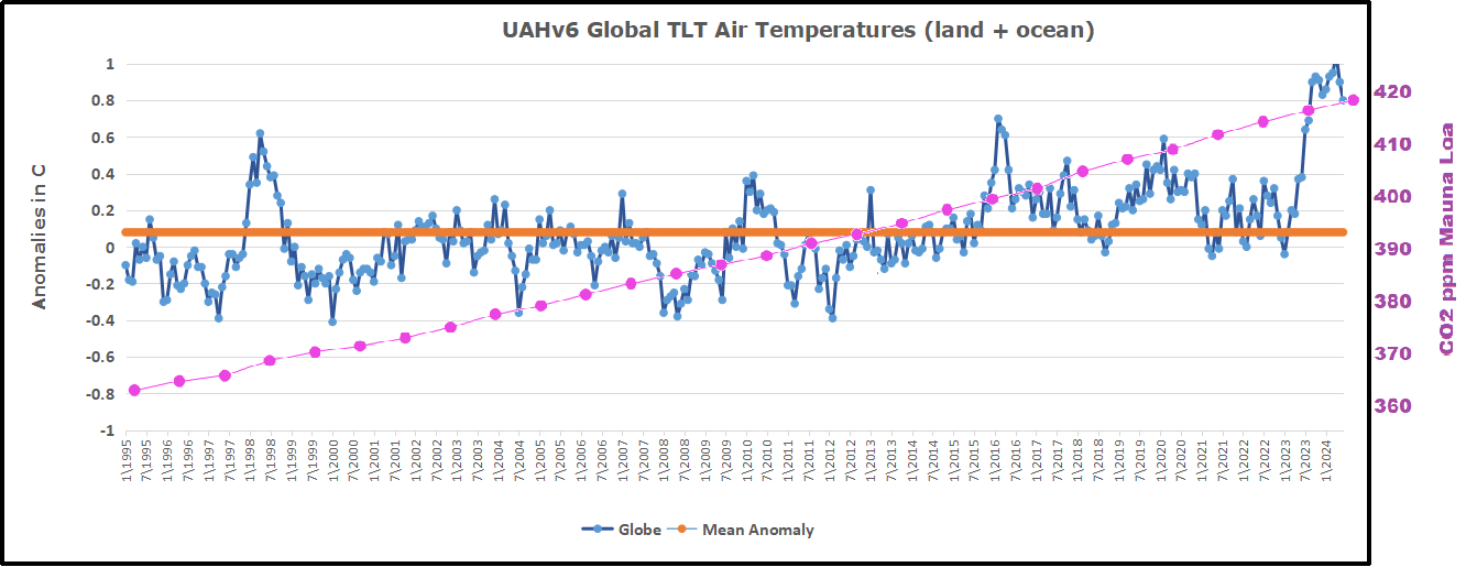
For reference I added an overlay of CO2 annual concentrations as measured at Mauna Loa.  While temperatures fluctuated up and down ending flat, CO2 went up steadily by ~60 ppm, a 15% increase.

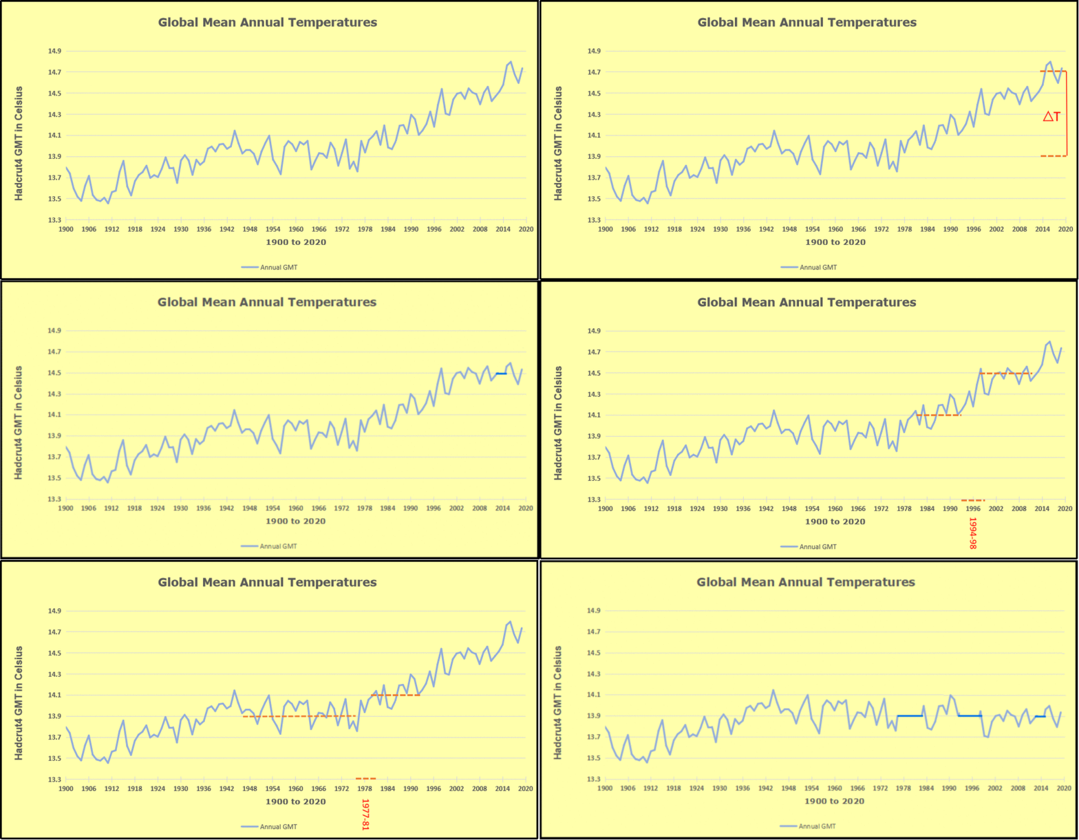
Furthermore, going back to previous warmings prior to the satellite record shows that the entire rise of 0.8C since 1947 is due to oceanic, not human activity.
gmt-warming-events

The animation is an update of a previous analysis from Dr. Murry Salby.  These graphs use Hadcrut4 and include the 2016 El Nino warming event.  The exhibit shows since 1947 GMT warmed by 0.8 C, from 13.9 to 14.7, as estimated by Hadcrut4.  This resulted from three natural warming events involving ocean cycles. The most recent rise 2013-16 lifted temperatures by 0.2C.  Previously the 1997-98 El Nino produced a plateau increase of 0.4C.  Before that, a rise from 1977-81 added 0.2C to start the warming since 1947.

Importantly, the theory of human-caused global warming asserts that increasing CO2 in the atmosphere changes the baseline and causes systemic warming in our climate.  On the contrary, all of the warming since 1947 was episodic, coming from three brief events associated with oceanic cycles. And now in 2024 we have seen an amazing episode with a temperature spike driven by ocean air warming in all regions, along with rising NH land temperatures, now dropping below its peak.

Chris Schoeneveld has produced a similar graph to the animation above, with a temperature series combining HadCRUT4 and UAH6. H/T WUWT
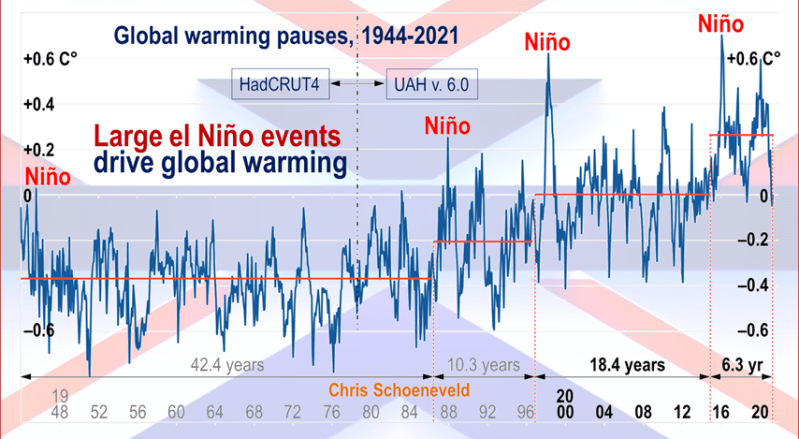
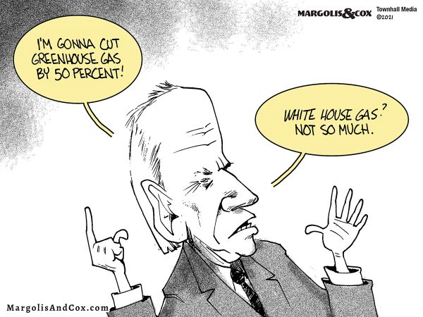
image-8


mc_wh_gas_web20210423124932

See Also Worst Threat: Greenhouse Gas or Quiet Sun?

December 2024 Ocean Leads Global Cooling banner-blog

With apologies to Paul Revere, this post is on the lookout for cooler weather with an eye on both the Land and the Sea.  While you heard a lot about 2020-21 temperatures matching 2016 as the highest ever, that spin ignores how fast the cooling set in.  The UAH data analyzed below shows that warming from the last El Nino had fully dissipated with chilly temperatures in all regions. After a warming blip in 2022, land and ocean temps dropped again with 2023 starting below the mean since 1995.  Spring and Summer 2023 saw a series of warmings, continuing into October, followed by cooling in November and December.

UAH has updated their TLT (temperatures in lower troposphere) dataset for December 2024. Due to one satellite drifting more than can be corrected, the dataset has been recalibrated and retitled as version 6.1 Graphs here contain this updated 6.1 data.  Posts on their reading of ocean air temps this month are ahead of the update from HadSST4.  I posted recently on SSTs Ocean Remains Cooler November 2024. These posts have a separate graph of land air temps because the comparisons and contrasts are interesting as we contemplate possible cooling in coming months and years.

Sometimes air temps over land diverge from ocean air changes. In July 2024 all oceans were unchanged except for Tropical warming, while all land regions rose slightly. In August we saw a warming leap in SH land, slight Land cooling elsewhere, a dip in Tropical Ocean temp and slightly elsewhere.  September showed a dramatic drop in SH land, overcome by a greater NH land increase. In October, ocean and land temps in both NH and Tropics dropped, pulling the global anomaly down. Now in November and December there was cooling everywhere, except only SH and Tropics land temps.

Note:  UAH has shifted their baseline from 1981-2010 to 1991-2020 beginning with January 2021.   v6.1 data was recalibrated also starting with 2021. In the charts below, the trends and fluctuations remain the same but the anomaly values changed with the baseline reference shift.

Presently sea surface temperatures (SST) are the best available indicator of heat content gained or lost from earth’s climate system.  Enthalpy is the thermodynamic term for total heat content in a system, and humidity differences in air parcels affect enthalpy.  Measuring water temperature directly avoids distorted impressions from air measurements.  In addition, ocean covers 71% of the planet surface and thus dominates surface temperature estimates.  Eventually we will likely have reliable means of recording water temperatures at depth.

Recently, Dr. Ole Humlum reported from his research that air temperatures lag 2-3 months behind changes in SST.  Thus cooling oceans portend cooling land air temperatures to follow.  He also observed that changes in CO2 atmospheric concentrations lag behind SST by 11-12 months.  This latter point is addressed in a previous post Who to Blame for Rising CO2?

After a change in priorities, updates are now exclusive to HadSST4.  For comparison we can also look at lower troposphere temperatures (TLT) from UAHv6.1 which are now posted for December.  The temperature record is derived from microwave sounding units (MSU) on board satellites like the one pictured above. Recently there was a change in UAH processing of satellite drift corrections, including dropping one platform which can no longer be corrected. The graphs below are taken from the revised and current dataset.

The UAH dataset includes temperature results for air above the oceans, and thus should be most comparable to the SSTs. There is the additional feature that ocean air temps avoid Urban Heat Islands (UHI).  The graph below shows monthly anomalies for ocean air temps since January 2015.
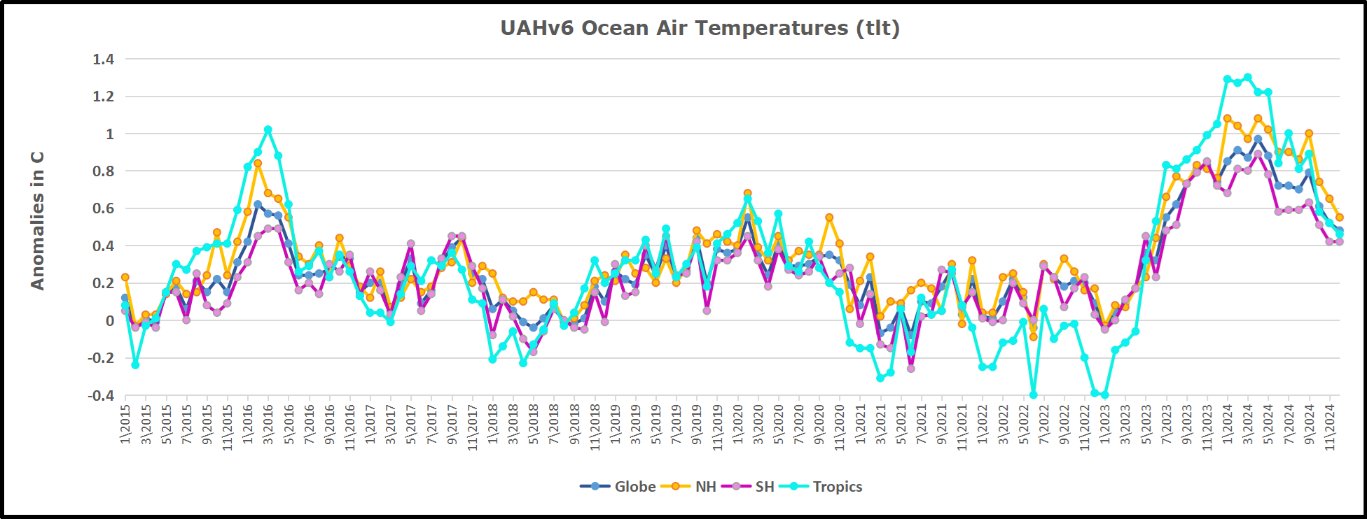
In 2021-22, SH and NH showed spikes up and down while the Tropics cooled dramatically, with some ups and downs, but hitting a new low in January 2023. At that point all regions were more or less in negative territory. 

After sharp cooling everywhere in January 2023, there was a remarkable spiking of Tropical ocean temps from -0.5C up to + 1.2C in January 2024.  The rise was matched by other regions in 2024, such that the Global anomaly peaked at 0.95C in May, Since then the Tropics and the Global anomaly have cooled down to 0.5C, as well as SH dropping down to 0.4C in December.

Land Air Temperatures Tracking in Seesaw Pattern

We sometimes overlook that in climate temperature records, while the oceans are measured directly with SSTs, land temps are measured only indirectly.  The land temperature records at surface stations sample air temps at 2 meters above ground.  UAH gives tlt anomalies for air over land separately from ocean air temps.  The graph updated for December is below.
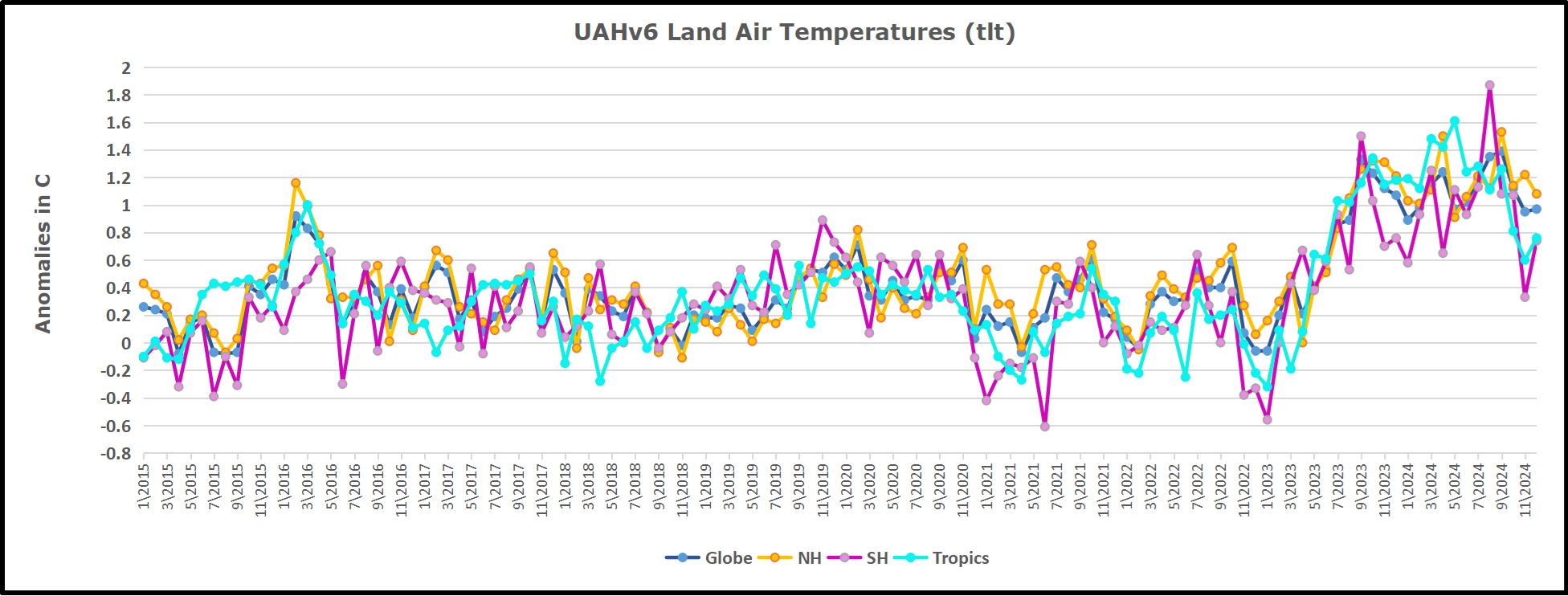
Here we have fresh evidence of the greater volatility of the Land temperatures, along with extraordinary departures by SH land.  The seesaw pattern in Land temps is similar to ocean temps 2021-22, except that SH is the outlier, hitting bottom in January 2023. Then exceptionally SH goes from -0.6C up to 1.4C in September 2023 and 1.8C in  August 2024, with a large drop in between.  In November, SH and the Tropics pulled the Global Land anomaly further down despite a bump in NH land temps. December showed an upward rebound in SH and Tropics land temps, offset by a NH drop, leaving the Global land anomaly little changed.

The Bigger Picture UAH Global Since 1980
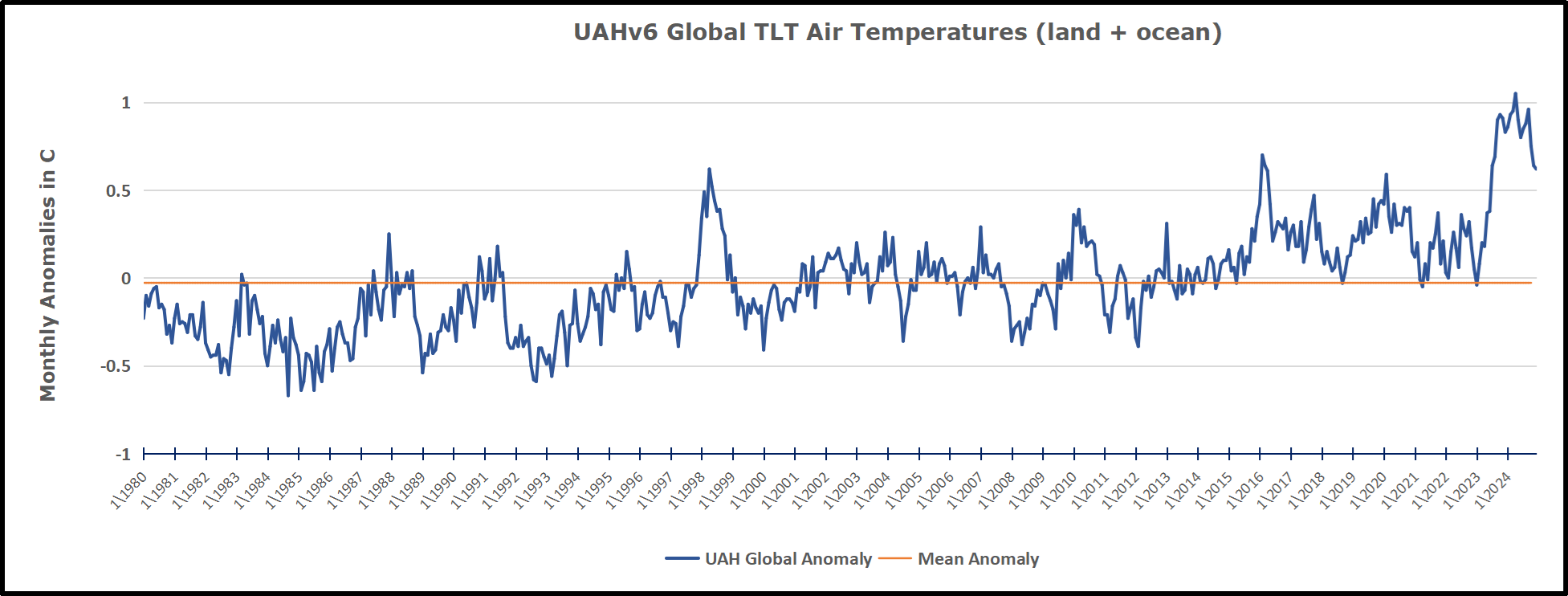
The chart shows monthly Global Land and Ocean anomalies starting 01/1980 to present.  The average monthly anomaly is -0.03, for this period of more than four decades.  The graph shows the 1998 El Nino after which the mean resumed, and again after the smaller 2010 event. The 2016 El Nino matched 1998 peak and in addition NH after effects lasted longer, followed by the NH warming 2019-20.   An upward bump in 2021 was reversed with temps having returned close to the mean as of 2/2022.  March and April brought warmer Global temps, later reversed

With the sharp drops in Nov., Dec. and January 2023 temps, there was no increase over 1980. Then in 2023 the buildup to the October/November peak exceeded the sharp April peak of the El Nino 1998 event. It also surpassed the February peak in 2016. In 2024 March and April took the Global anomaly to a new peak of 0.94C.  The cool down started with May dropping to 0.9C, and in June a further decline to 0.8C.  October went down to 0.7C,  November and December dropped to 0.6C. 

The graph reminds of another chart showing the abrupt ejection of humid air from Hunga Tonga eruption.
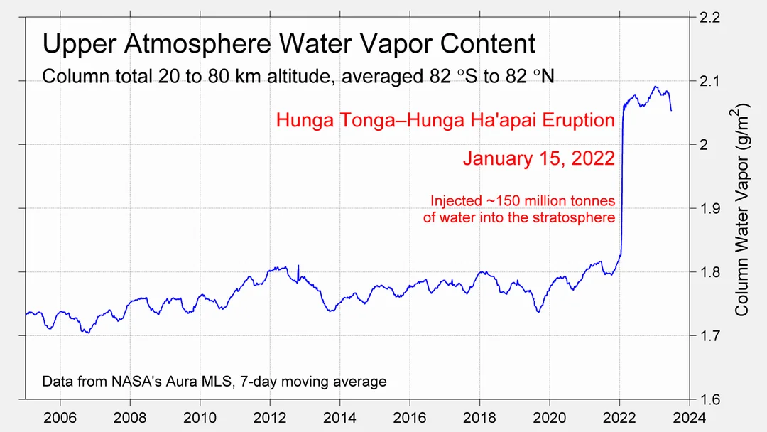
TLTs include mixing above the oceans and probably some influence from nearby more volatile land temps.  Clearly NH and Global land temps have been dropping in a seesaw pattern, nearly 1C lower than the 2016 peak.  Since the ocean has 1000 times the heat capacity as the atmosphere, that cooling is a significant driving force.  TLT measures started the recent cooling later than SSTs from HadSST4, but are now showing the same pattern. Despite the three El Ninos, their warming had not persisted prior to 2023, and without them it would probably have cooled since 1995.  Of course, the future has not yet been written.


via Science Matters

https://ift.tt/NhOkf6D

January 3, 2025 at 05:27PM

New York Response to Part 490 Sea-Level Rise Amendment Comments

Roger Caiazza

This is an update to some articles that were published early in 2024 about the New York State Department of Environmental Conservation (DEC) proposed Amendments to Part 490, Projected Sea Level Rise (Amendment).  Kip Hansen wrote a post entitled New York State Sea Level Rise:  Fantasy as Law.   A few days later Anthony Watts responded to a New York Post article by Carl Campanile with the headline: Sea levels around NYC could surge up to 13 inches in 2030s due to climate change: state study. I prepared comments which I summarized in a post.  In September 2024 DEC adopted the Amendment.  Surprising no one, their Assessment of Public Comments blew off all the concerns expressed.  

Part 490 Projected Sea-Level Rise

DEC’s Climate Change Regulatory Revisions webpage describes the Amendment to the regulation:

On September 22, 2014, the Community Risk and Resiliency Act was signed into law — Chapter 355 of the Laws of 2014 (CRRA). CRRA is intended to ensure that decisions regarding certain State permits and expenditures consider climate risk, including sea-level rise. Among other things, CRRA requires the Department of Environmental Conservation (Department) to adopt regulations establishing science-based State sea-level rise projections. Therefore, the Department proposed a new 6 NYCRR Part 490, Projected Sea-Level Rise (Part 490). Part 490 establishes projections of sea-level rise in three specified geographic regions over various time intervals, but does not impose any requirements on any entity. An amended Part 490 was adopted in September 2024 with no revisions to the draft released for public comment in January 2024.

Kip Hansen summarized New York sea level rise history and the DEC projections in detail in his post.  What you need to know here is that New York City’s sea level has been increasing 3 mm per year over 167 years.  Enough of that observed increase is caused by local subsidence so that the remainder is “very close to the standardly cited Global Sea Level Rise figure for the 20th Century of 1.7 or 1.8 mm/yr.  (opinions vary – see NOAA here.)”   Kip explains that the projected increases included in the Amendment” have not been seen in the decade since the 2014 update report and, based on the historical record, are extremely unlikely to be seen in the near future.” He points out that “all the projections, in the Amendment, in the NYSERDA 2014 report and in the NYS Climate Assessment require doubling and tripling of long-term sea-level rise rates in New York City.”

RCP8.5 Comments

Kip, Anthony, and I agree that the projections are flawed because the methodology estimates an unrealistically high projected sea-level dependent upon an impossible climate model scenario.  Depending upon which version of the Intergovernmental Panel on Climate Change report being used the modeling scenarios are known either as a Representative Concentration Pathway (RCP) or Shared Socio-economic Pathways (SSP).  The RCP-8.5 scenario has been debunked by many as Anthony reported here and here.  My comments focused on the misuse of RCP-8.5 using some of those references and adding others. 

The Amendment revises the projections of future sea-level rise required by New York regulations. 

I raised the RCP-8.5 concerns in the pre-proposal draft of the amendment.  The Regulatory Impact Statement (RIS) uses the label SSP5-8.5 for this scenario and admits that those emission scenarios are implausible:

The Department acknowledges that current GHG emissions policies would result in actual emissions lower than projected by SSP5-8.5. Thus, the inclusion of higher projections of sea level rise, especially those based on SSP5-8.5, could lead to consideration of conditions that are unlikely to occur, at least in the more immediate future.

So how did DEC justify the continued use of SSP5-8.5?  The RIS goes to considerable lengths to justify its use with statements like the following: “Unfortunately, current literature does not provide a basis for assessment of the emissions levels at which ice shelf and marine ice cliff instability, important factors in sea level rise in high emissions scenarios, such as SSP5-8.5, become significant.” 

Response to RCP8.5 Comments

DEC is required to respond to submitted comments.  The Assessment of Public Comments document addressed my arguments in their response to Comment 6.  They summarized my concerns saying that “SSP5-8.5 is not plausible, and model outputs based on this SSP, including the rapid ice melt scenario, should not be included in the projections.”   The reply stated:

Response to Comment 6: DEC has described its rationale for including SSP5-8.5 model outputs in its projections, including the rapid ice melt scenario, in the RIS. To summarize here, the emission-reduction gap noted above, uncertainties in the causal chain to sea level heights, including ice cliff and ice shelf stability, and reports of accelerating Antarctic and Greenland ice loss reduce confidence that SLR will be limited to the levels projected by SSP2-4.5 models.  The CIA methodology report (p. 21) provides additional rationale for including projections based on SSP5-8.5:

• Continuity with previous New York State projections, which were based on representative concentration pathways with the same end-of-century radiative forcing.

• Stakeholder interest in these projections, based on CIA Needs Assessment.

• Value of identifying a broad range of plausible outcomes.

• Current climate impact models’ underestimation of plausible outcomes when driven by only moderate GHG forcing.

DEC maintains that inclusion of high, albeit unlikely, projections to enable consideration of the consequences of low-probability but high-consequence events to be the more prudent alternative to limiting projections to those based on SSP2-4.5.

The crux of my disagreement is the value of incorporating what is essentially an impossible scenario.  All the reasons cited attempt to justify what is essentially an executive decision to perpetuate the narrative that there is an existential threat of climate change exemplified, in this case, by extraordinary sea-level rise projections. 

It is telling that the response claims that the extreme projections are included because of “Stakeholder interest in these projections, based on CIA Needs Assessment.”  New York State agencies love to claim that they have a robust stakeholder process.  However, the stakeholder process operates with a loaded deck.  The New York Research & Development Authority (NYSEDA) CIA Needs Assessment Steering Committee is a relevant example.  The report states “The assessment has been guided by a Steering Committee of climate scientists, assessment experts, and representatives from nonprofit organizations and state and municipal government agencies.”  I am very critical of the review process because I know that there is immense pressure to adhere to the narrative within NYSERDA and I am sure no one skeptical of the extreme impact narrative was allowed anywhere near the Steering Committee. In addition, technical analyses performed for NYSERDA will not be funded in the future if the answers do not support the narrative.

Another reason given for using the impossible scenario is the “value of identifying broad outcomes”.  In this instance I think the value is primarily for the “scare the bejesus out of the populace” narrative needed to perpetuate the story that New York politicians are here to save the planet even in the face of increasingly obvious enormous costs, threats to reliability, and inevitable reduction in personal choice.  This will only stop when there is a change in the political balance of New York.

Conclusion

Surprising no one, their Assessment of Public Comments blew off our concerns.  There is no reasonable defense for using RCP-8.5.  As long as New York State continues to claim they follow the science but ignore it when it is inconvenient, the more likely the rush to the bottom will become a death spiral. 


Roger Caiazza blogs on New York energy and environmental issues at Pragmatic Environmentalist of New York.  This represents his opinion and not the opinion of any of his previous employers or any other organization with which he has been associated.


Discover more from Watts Up With That?

Subscribe to get the latest posts sent to your email.

via Watts Up With That?

https://ift.tt/lhbr1Sk

January 3, 2025 at 04:07PM

The UK pays wind turbines for failure — so the market wants to install more failures

AI generated. Wind turbine leeches.

Subsidy farms are designed to suck payments from plumbers, bakers and mums and dads.

By Jo Nova

When failure becomes a commodity…

Ponder for a moment how intrinsically unsuitable, maladapted, and worthless wind turbines are to a grid. Their failure is so comprehensive, multifaceted and inevitable, an entirely new and bizarre market was invented to reward their failures. Even when they generate electricity, if the time is wrong, the demand is low, or the network can’t handle it, they will still be paid. The grid can’t use the power, but the customer still gets slugged for something they didn’t use, or they couldn’t get. In the UK the costs for this useless power grew to nearly £400 million last year.

The largest provider of useless power was SeaGreen wind plant which made nearly twice as much from being “constrained” than from being of service. The Renewable Energy Foundation (REF) reports that SeaGreen earned £100 million for making electricity, and £200 million for being “constrained”. Effectively, the useful electricity it made costs a shocking £2.70 a kilowatt hour, after the other payments are included.

Obviously, when the government rewards failure, the market responds by planning to fail. It follows then that industrial wind plant developers would be bonkers if they weren’t looking for sites where their output would arrive at the worst possible time, or through the most remote and overloaded corner of the network.

Everything about the wind industry has “Rent Seeker” tattooed all over it.

Campaign group Net Zero Watch has condemned the renewables industry rip-off of electricity consumers. New data published by the Renewable Energy Foundation reveals that the cost of paying windfarms to switch off soared by 91% in 2024. These payments are necessary when the grid has insufficient capacity to deliver the power to market. Nearly £400 million was paid to windfarms in 2024, and much more than this in indirect costs [1].

The largest single recipient was Seagreen, a new windfarm off the coast of Angus, which received nearly £200 million in these so-called “constraint payments”.

Net Zero Watch director Andrew Montford said:

The Renewable Energy Foundation suggest that Seagreen is making around £270 for each megawatt hour it actually produces, more than three times market averages, because it’s so lucrative to be switched off. This is a truly obscene rip-off of the consumer.

Windfarms seem to be being deliberately built in Scottish waters, where they will receive lucrative payments to be switched off.

And there are huge numbers of new windfarms planned for Scottish waters, where they will be just as constrained. So the rip-off is only going to get worse.

[1] When windfarms have to switch off, their customers still need power, so it is necessary to pay a gas-fired power station to switch on to meet demand.

SeaGreen wind plant has about 114 towers in the ocean east of Scotland. It could make about 1 gigawatt in theoretical capacity if all the turbines were working, but its actual load factor was a pathetic 14%. Of course, as a subsidy farm, it’s load factor was 200%.

Imagine a coal plant that earned money every time it had to slow down because customers weren’t using as much electricity as the power plant could have made?

h/t to Andrew Montford @Dissentient

0 out of 10 based on 0 rating

via JoNova

https://ift.tt/wUPNEDR

January 3, 2025 at 02:37PM

Lacking Data, Climate Models Rely on Guesses

A recent question was posed on  Quora: Say there are merely 15 variables involved in predicting global climate change. Assume climatologists have mastered each variable to a near perfect accuracy of 95%. How accurate would a climate model built on this simplified system be?  Keith Minor has a PhD in organic chemistry, PhD in Geology, and PhD in Geology & Paleontology from The University of Texas at Austin.  He responded with the text posted below in italics with my bolds and added images.

I like the answers to this question, and Matthew stole my thunder on the climate models not being statistical models. If we take the question and it’s assumptions at face value, one unsolvable overriding problem, and a limit to developing an accurate climate model that is rarely ever addressed, is the sampling issue. Knowing 15 parameters to 99+% accuracy won’t solve this problem.

The modeling of the atmosphere is a boundary condition problem. No, I’m not talking about frontal boundaries. Thermodynamic systems are boundary condition problems, meaning that the evolution of a thermodynamic system is dependent not only on the conditions at t > 0 (is the system under adiabatic conditions, isothermal conditions, do these conditions change during the process, etc.?), but also on the initial conditions at t = 0 (sec, whatever). Knowing almost nothing about what even a fraction of a fraction of the molecules in the atmosphere are doing at t = 0 or at t > 0 is a huge problem to accurately predicting what the atmosphere will do in the near or far future. [See footnote at end on this issue.]

Edward Lorenz attempted to model the thermodynamic behavior of the atmosphere by using models that took into account twelve variables (instead of fifteen as posed by the questioner), and found (not surprisingly) that there was a large variability in the models. Seemingly inconsequential perturbations would lead to drastically different results, which diverged (euphemism for “got even worse”) the longer out in time the models were run (they still do). This presumably is the origin of Lorenz’s phrase “the butterfly effect”. He probably meant it to be taken more as an instructive hypothetical rather than a literal effect, as it is too often taken today. He was merely illustrating the sensitivity of the system to the values of the parameters, and not equating it to the probability of outcomes, chaos theory, etc., which is how the term has come to be known. This divergence over time is bad for climate models, which try to predict the climate decades from now. Just look at the divergence of hurricane “spaghetti” models, which operate on a multiple-week scale.

The sources of variability include:

♦  the inability of the models to handle water (the most important greenhouse gas in the atmosphere, not CO2) and processes related to it;

♦  e.g., models still can’t handle the formation and non-formation of clouds;
♦  the non-linearity of thermodynamic properties of matter (which seem to be an afterthought, especially in popular discussions regarding the roles that CO2 plays in the atmosphere and biosphere), and
♦  the always-present sampling problem.

While in theory it is possible to know what a statistically significant number of the air and water molecules are doing at any point in time (that would be a lot of atoms and molecules!), a statistically significant sample of air molecules is certainly not being sampled by releasing balloons twice a day from 90 some odd weather stations in the US and territories, plus the data from commercial aircraft, plus all of the weather data from around the World. Doubling this number wouldn’t help, i.e wouldn’t make any difference. Though there are some blind spots, such as northeast Texas that might benefit from having a radar in the area. So you have to weigh the cost of sampling more of the atmosphere versus the 0% increase in forecasting accuracy (within experimental error) that you would get by doing so.

I’ll go out on a limb and say that the NWS (National Weather Service) is actually doing pretty good job in their 5-day forecasts with the current data and technologies that they have (e.g., S-band radar), and the local meteorologists use their years of experience and judgment to refine the forecasts to their viewing areas. The old joke is that a meteorologist’s job is the one job where you can be wrong more than half the time and still keep your job, but everyone knows that they go to work most, if not all, days with one hand tied behind their back, and sometimes two! The forecasts are not that far off on average, and so meteorologists get my unconditional respect.

In spite of these daunting challenges, there are certainly a number of areas in weather forecasting that can be improved by increased sampling, especially on a local scale. For example, for severe weather outbreaks, the CASA project is being implemented using multiple, shorter range radars that can get multiple scan directions on nearby severe-warned cells simultaneously. This resolves the problem caused by the curvature of the Earth as well as other problems associated with detecting storm-scale features tens or hundreds of miles away from the radar. So high winds, hail, and tornadoes are weather events where increasing the local sampling density/rate might help improve both the models and forecasts.

Prof. Wurman at OU has been doing this for decades with his pioneering work with mobile radar (the so-called “DOW’s”). Let’s not leave out the other researchers who have also been doing this for decades. The strategy of collecting data on a storm from multiple directions at short distances, coupled with supercomputer capabilities, has been paying off for a number of years. As a recent example, Prof. Orf at UW Madison, with his simulation of the May 24th, 2011 El Reno, OK tornado (you’ve probably seen it on the Internet), has shed light on some of the “black box” aspects to how tornadoes form. [Video below is Leigh Orf 1.5 min segment for 2018 Blue Waters Symposium plenary session. This segment summarizes, in 90 seconds, some of the team’s accomplishments on the Blue Waters supercomputer over the past five years.

Prof. Orf’s simulation is just that, and the resolution is around ~10 m (~33 feet), but it illustrates how increased targeted sampling can be effective in at least understanding the complex, thermodynamic processes occurring within a storm. Colleagues have argued that the small improvements in warning times in the last couple of decades are really due more to the heavy spotter presence these days rather than case studies of severe storms. That may be true. However, in test cases of the CASA system, it picked out the subtle boundaries along which the storms fired that did go unnoticed with the current network of radars. So I’m optimistic about increased targeted sampling for use in an early warning system.

These two examples bring up a related problem-too much data! As commented on by a local meteorologist at a TESSA meeting, one of the issues with CASA that will have to be resolved is how to handle/process the tremendous amounts of data that will be generated during a severe weather outbreak. This is different from a research project where you can take your data back to the “lab”. In a real-time system, such as CASA, you need to have the ability to process the volumes of data rapidly so a meteorologist can quickly make a decision and get that life-saving info to the public. This data volume issue may be less of a problem for those using the data to develop climate models.

So back to the Quora question, with regard to a cost-effective (cost-effect is the operational term) climate model or models (say an ensemble model) that would “verify” say 50 years from now, the sampling issue is ever present, and likely cost-prohibitive at the level needed to make the sampling statistically significant. And will the climatologist be around in 50 years to be “hoisted with their own petard” when the climate model is proven to be wrong? The absence of accountability is the other problem with these long-range models into which many put so much faith.

But don’t stop using or trying to develop better climate models. Just be aware of what variables they include, how well they handle the parameters, and what their limitations are. How accurate would a climate model built on this simplified system [edit: of 15 well-defined variables (to 95% confidence level)] be? Not very!

My Comment

As Dr. Minor explains, powerful modern computers can process detailed observation data to simulate and forecast storm activity.  There are more such tools for preparing and adapting to extreme weather events which are normal in our climate system and beyond our control.  He also explains why long-range global climate models presently have major limitations for use by policymakers.

Footnote Regarding Initial Conditions Problem

What About the Double Pendulum?

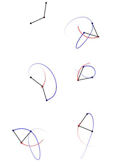
Trajectories of a double pendulum

A comment by tom0mason at alerted me to the science demonstrated by the double compound pendulum, that is, a second pendulum attached to the ball of the first one. It consists entirely of two simple objects functioning as pendulums, only now each is influenced by the behavior of the other.

Lo and behold, you observe that a double pendulum in motion produces chaotic behavior. In a remarkable achievement, complex equations have been developed that can and do predict the positions of the two balls over time, so in fact the movements are not truly chaotic, but with considerable effort can be determined. The equations and descriptions are at Wikipedia Double Pendulum

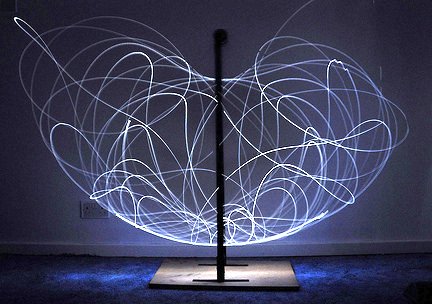
Long exposure of double pendulum exhibiting chaotic motion (tracked with an LED)

But here is the kicker, as described in tomomason’s comment:

If you arrive to observe the double pendulum at an arbitrary time after the motion has started from an unknown condition (unknown height, initial force, etc) you will be very taxed mathematically to predict where in space the pendulum will move to next, on a second to second basis. Indeed it would take considerable time and many iterative calculations (preferably on a super-computer) to be able to perform this feat. And all this on a very basic system of known elementary mechanics.

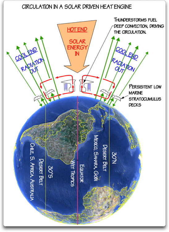
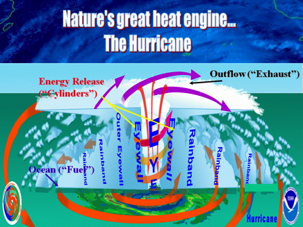
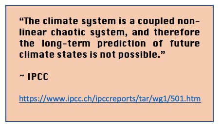
Our Chaotic Climate System


via Science Matters

https://ift.tt/GRrbu0W

January 3, 2025 at 01:26PM