Daily News 6 Nov 2024

Trump’s Victory and Climate Policy

While climate policy wasn’t the star of this recent election, the results carry significant implications for the climate agenda. Voters weren’t casting ballots explicitly for or against green energy mandates, net-zero goals, or climate “emergencies.” Yet, indirectly, they sent a strong signal: the public isn’t fully buying into the costly, disruptive climate policies that have become a pillar of certain political platforms. As the dust settles, the reality is clear—the green agenda just lost substantial footing, and its backers will have to reckon with what that means moving forward.

Climate Policy as a Secondary Issue with Primary Ramifications

It’s true; voters in this election were concerned primarily with issues closer to home—economic stability, inflation, job security, and immediate energy costs. But even as climate policy took a back seat in the campaign discourse, its implications loomed in the background. In states where green mandates have been most aggressive, energy prices have soared, job sectors have been strained, and the promise of renewable jobs hasn’t materialized to the extent promised. These factors, while not always top-of-mind in election messaging, have clearly made an impression on the public.

What we’re seeing is a kind of indirect referendum on the climate policies that have dominated recent years. Voters may not have explicitly voted on green policies, but the growing awareness of the trade-offs involved is unmistakable. The failure of candidates most closely aligned with aggressive climate agendas shows an implicit but impactful rejection of policies that prioritize carbon cuts and renewables at the expense of reliable, affordable energy.

The Green Agenda Takes a Back Seat

For years, climate alarmism has driven policy without substantial public scrutiny. Climate mandates were passed through sweeping bills, and green energy was sold as the inevitable future. However, this election signals a turning point. The quiet but firm message from voters was that climate goals can’t overrun practical concerns, especially as they impact household budgets and energy security.

The hard truth is this: while voters might generally support the idea of a cleaner environment, they’re clearly unwilling to shoulder the disruptive and costly consequences that come with rushed climate policies. Skyrocketing energy bills, faltering grid reliability, and the disappearance of traditional energy jobs are realities that weigh heavily on ordinary Americans. People may want a healthy planet, but they also want heat in the winter, affordable gas, and the economic security that has long come from stable energy industries.

The Implications for Policymakers

For climate policymakers, this election result is a wake-up call to recalibrate. The defeat of the green agenda in the background of these results reveals the limits of popular patience for top-down mandates that affect daily life. If lawmakers are paying attention, they’ll see that policies need to be practical, affordable, and adaptable, not dictated by climate scenarios that, however dire they may sound, lack resonance with the average voter’s immediate concerns.

In a way, this setback offers policymakers a chance to focus on balanced, flexible environmental strategies that don’t overburden citizens. The public’s quiet rejection of extreme climate policy can become an opportunity to develop approaches grounded in technological innovation, market-driven solutions, and gradual, economically viable transitions.

The Rise of Climate Realism

What this election suggests is that the era of unchecked climate alarmism may be shifting toward a more pragmatic, “climate realist” approach. Without overtly campaigning against green policies, voters have essentially said they’re not ready to make the kinds of sacrifices these policies demand. They’re looking for solutions that work with, not against, economic realities.

For the climate realist movement, these results represent a subtle but notable victory. The public has, in effect, rejected the notion that immediate, radical changes are the only solution to climate challenges. Instead, the message seems to be: take a measured approach, one that respects economic priorities and job security while still working toward environmental improvements.

A New Path Forward

As we look to the future, it’s evident that climate policy advocates must adjust their strategies. The message from the voting booth is unmistakable: the electorate is open to responsible environmental policy but weary of climate policies that impose financial strain without clear, tangible benefits. The public’s voice in this election suggests they’d rather see a steady, innovation-driven approach that strengthens—rather than weakens—their communities and the economy.

This election, though not explicitly about climate, may go down as a turning point for climate policy itself. Voters signaled that they won’t accept environmental goals at any cost, especially when that cost is borne by the average household. It’s a call for a shift from alarmist narratives to a practical, results-driven approach that respects both the environment and the economy.

via Watts Up With That?

https://ift.tt/McmDq2O

November 6, 2024 at 12:05PM

Daily News 6 Nov 2024

Climate Averages Reporting Stations.

https://www.metoffice.gov.uk/research/climate/maps-and-data/uk-climate-averages

In my letter to Peter Kyle Secretary of State for Science, Innovation and Technology I emphasized the “climate averages” quoted for many sites that no longer exist. Subsequently, many have asked for confirmations of these non-existent stations which I provide below.

Firstly the headline map is from the Met Office’s website initial screen detailing these climate average stations which are searchable on the above link either by name or clicking on the map. This is an example of what the supplied data for a station looks like. Coltishall is in Norfolk and closed 4/4/2006.

Note location, elevation and site nature is quoted with no indication given that it is no longer operational for climate reporting purposes and has not been so for 18 years.

If there is any doubt as to the closure of Coltishall, here is the current Google aerial image of the site with the red kite using Met Office supplied location co-ordinates. This former RAF site has been repurposed as a solar farm. Coltishall is number 79 on the list.

Below is the list as supplied under Freedom of Information request numbered IMS0211642 from the Met Office. It clearly states the “Open” or “Closed” status of each station with quoted “Climate Averages” on the above Met Office web page.

via Tallbloke’s Talkshop

https://ift.tt/RxBK9XP

November 6, 2024 at 11:01AM

Daily News 6 Nov 2024

10/2024 Update Recent Warming Spike Drives Rise in CO2

Previously I have demonstrated that changes in atmospheric CO2 levels follow changes in Global Mean Temperatures (GMT) as shown by satellite measurements from University of Alabama at Huntsville (UAH). That background post is reprinted later below.

My curiosity was piqued by the remarkable GMT spike starting in January 2023 and rising to a peak in April 2024. I also became aware that UAH has recalibrated their dataset due to a satellite drift that can no longer be corrected. The values since 2020 have shifted slightly in version 6.1, as shown in my report yesterday UAH October 2024: NH and Tropics Lead Global Cooling.

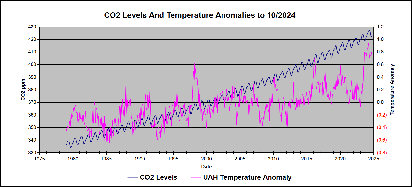
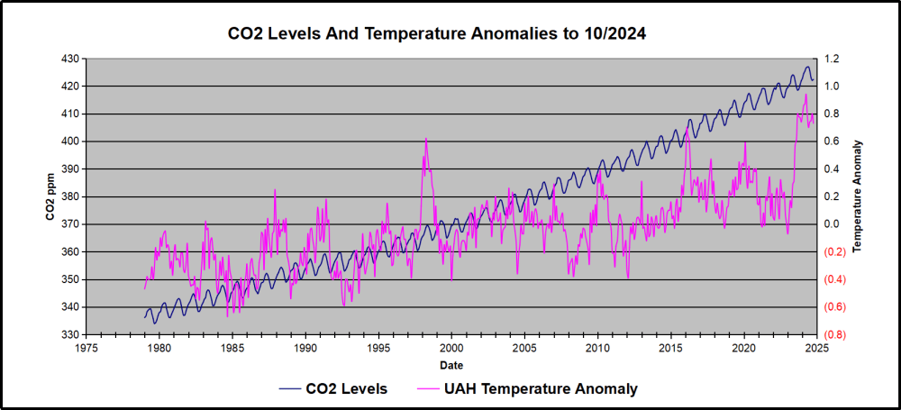
In this post, I test the premise that temperature changes are predictive of changes in atmospheric CO2 concentrations. The chart above shows the two monthly datasets: CO2 levels in blue reported at Mauna Loa, and Global temperature anomalies reported by UAHv6.1, both up to October 2024. Would such a sharp increase in temperature be reflected in rising CO2 levels, according to the successful mathematical forecasting model?

The answer is yes: that temperature spike results
in a corresponding CO2 spike as expected.

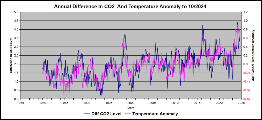
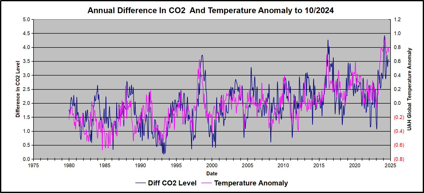
Above are UAH temperature anomalies compared to CO2 monthly changes year over year.

Changes in monthly CO2 synchronize with temperature fluctuations, which for UAH are anomalies now referenced to the 1991-2020 period. CO2 differentials are calculated for the present month by subtracting the value for the same month in the previous year (for example October 2024 minus October 2023). Temp anomalies are calculated by comparing the present month with the baseline month. Note the recent CO2 upward spike and drop following the temperature spike and drop.

The final proof that CO2 follows temperature due to stimulation of natural CO2 reservoirs is demonstrated by the ability to calculate CO2 levels since 1979 with a simple mathematical formula:

For each subsequent year, the co2 level for each month was generated

CO2 _{this month this year} = a + b × Temp _{this month this year} + CO2 _{this month last year}

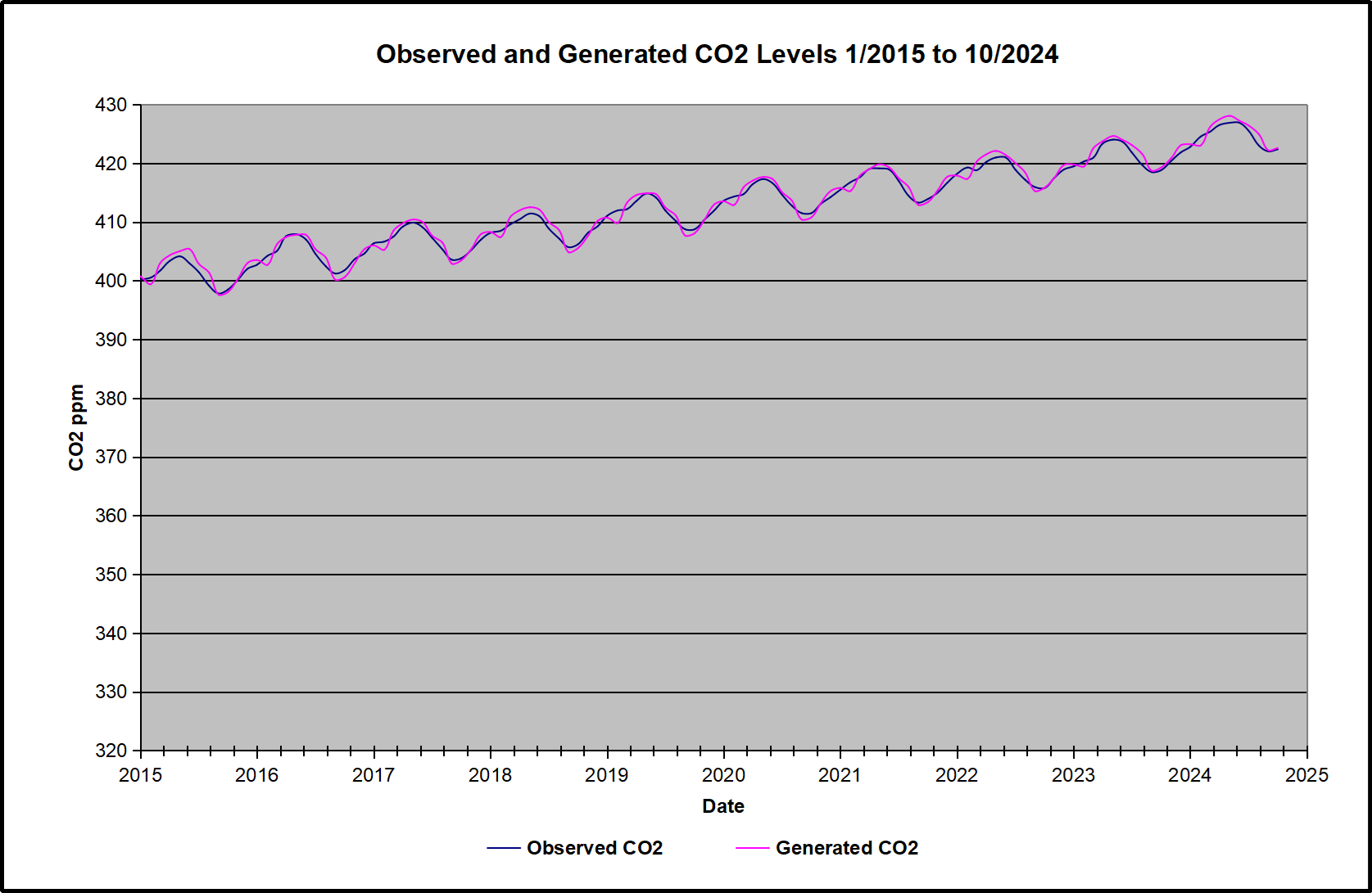
The values for a and b are constants applied to all monthly temps, and are chosen to scale the forecasted CO2 level for comparison with the observed value. Here is the result of those calculations.

In the chart calculated CO2 levels correlate with observed CO2 levels at 0.9987 out of 1.0000. This mathematical generation of CO2 atmospheric levels is only possible if they are driven by temperature-dependent natural sources, and not by human emissions which are small in comparison, rise steadily and monotonically. For a more detailed look at the recent fluxes, here are the results since 2015, an ENSO neutral year.

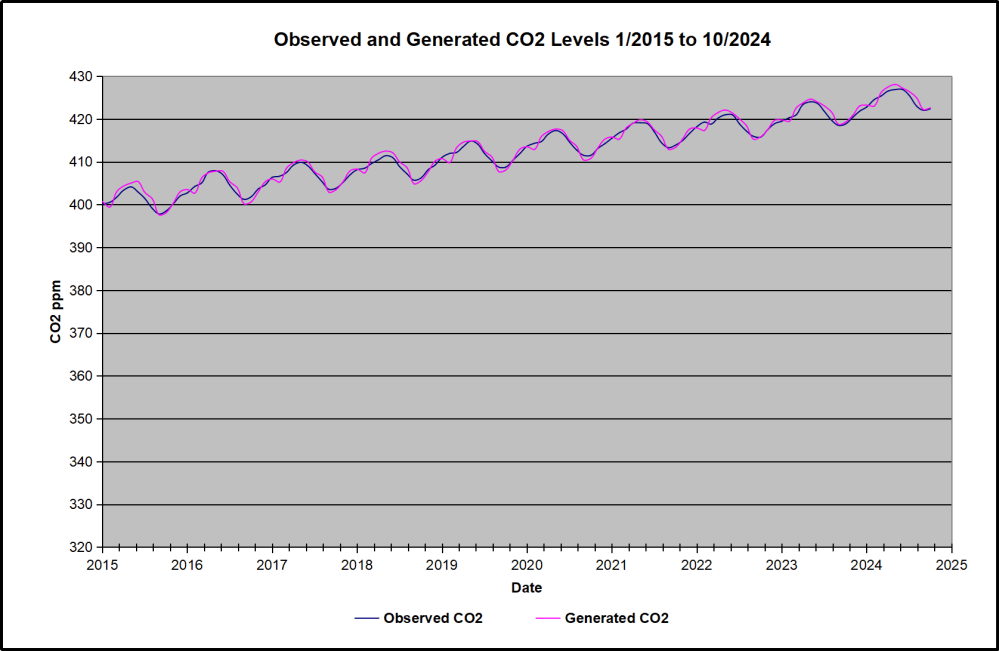
For this recent period, the calculated CO2 values match the annual lows, while some annual generated values of CO2 are slightly higher or lower than observed at other months of the year. Still the correlation for this period is 0.9928.

Key Point

Changes in CO2 follow changes in global temperatures on all time scales, from last month’s observations to ice core datasets spanning millennia. Since CO2 is the lagging variable, it cannot logically be the cause of temperature, the leading variable. It is folly to imagine that by reducing human emissions of CO2, we can change global temperatures, which are obviously driven by other factors.

Background Post Temperature Changes Cause CO2 Changes, Not the Reverse

This post is about proving that CO2 changes in response to temperature changes, not the other way around, as is often claimed. In order to do that we need two datasets: one for measurements of changes in atmospheric CO2 concentrations over time and one for estimates of Global Mean Temperature changes over time.

Climate science is unsettling because past data are not fixed, but change later on. I ran into this previously and now again in 2021 and 2022 when I set out to update an analysis done in 2014 by Jeremy Shiers (discussed in a previous post reprinted at the end). Jeremy provided a spreadsheet in his essay Murray Salby Showed CO2 Follows Temperature Now You Can Too posted in January 2014. I downloaded his spreadsheet intending to bring the analysis up to the present to see if the results hold up. The two sources of data were:

Temperature anomalies from RSS here: http://www.remss.com/missions/amsu

CO2 monthly levels from NOAA (Mauna Loa): https://www.esrl.noaa.gov/gmd/ccgg/trends/data.html

Changes in CO2 (ΔCO2)

Uploading the CO2 dataset showed that many numbers had changed (why?).

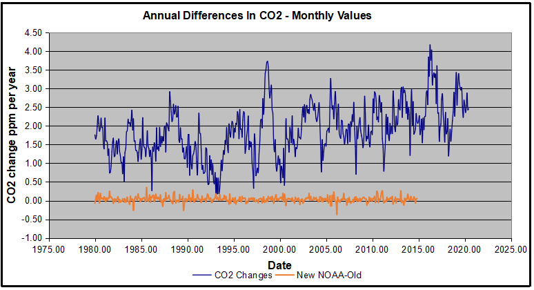
The blue line shows annual observed differences in monthly values year over year, e.g. June 2020 minus June 2019 etc. The first 12 months (1979) provide the observed starting values from which differentials are calculated. The orange line shows those CO2 values changed slightly in the 2020 dataset vs. the 2014 dataset, on average +0.035 ppm. But there is no pattern or trend added, and deviations vary randomly between + and -. So last year I took the 2020 dataset to replace the older one for updating the analysis.

Now I find the NOAA dataset starting in 2021 has almost completely new values due to a method shift in February 2021, requiring a recalibration of all previous measurements. The new picture of ΔCO2 is graphed below.

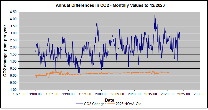
The method shift is reported at a NOAA Global Monitoring Laboratory webpage, Carbon Dioxide (CO2) WMO Scale, with a justification for the difference between X2007 results and the new results from X2019 now in force. The orange line shows that the shift has resulted in higher values, especially early on and a general slightly increasing trend over time. However, these are small variations at the decimal level on values 340 and above. Further, the graph shows that yearly differentials month by month are virtually the same as before. Thus I redid the analysis with the new values.

Global Temperature Anomalies (ΔTemp)

The other time series was the record of global temperature anomalies according to RSS. The current RSS dataset is not at all the same as the past.

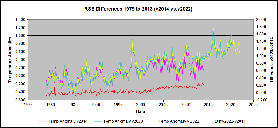
Here we see some seriously unsettling science at work. The purple line is RSS in 2014, and the blue is RSS as of 2020. Some further increases appear in the gold 2022 rss dataset. The red line shows alterations from the old to the new. There is a slight cooling of the data in the beginning years, then the three versions mostly match until 1997, when systematic warming enters the record. From 1997/5 to 2003/12 the average anomaly increases by 0.04C. After 2004/1 to 2012/8 the average increase is 0.15C. At the end from 2012/9 to 2013/12, the average anomaly was higher by 0.21. The 2022 version added slight warming over 2020 values.

RSS continues that accelerated warming to the present, but it cannot be trusted. And who knows what the numbers will be a few years down the line? As Dr. Ole Humlum said some years ago (regarding Gistemp): “It should however be noted, that a temperature record which keeps on changing the past hardly can qualify as being correct.”

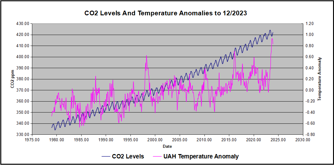
Given the above manipulations, I went instead to the other satellite dataset UAH version 6. UAH has also made a shift by changing its baseline from 1981-2010 to 1991-2020. This resulted in systematically reducing the anomaly values, but did not alter the pattern of variation over time. For comparison, here are the two records with measurements through December 2023.

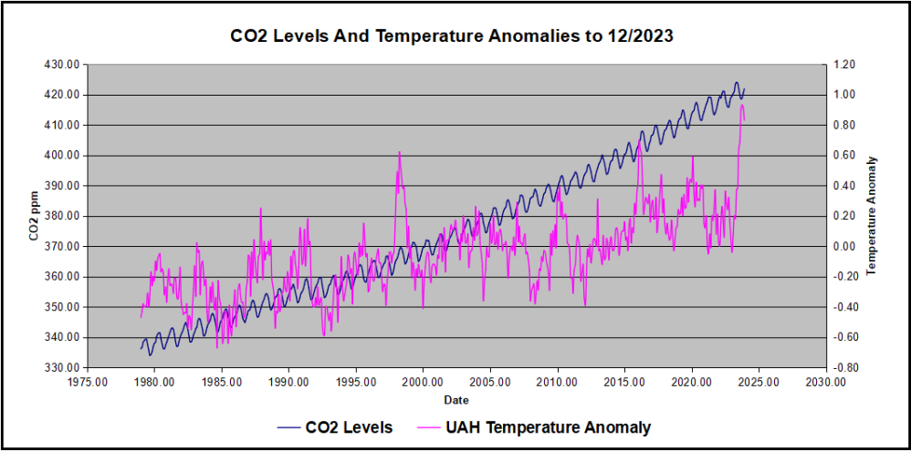
Comparing UAH temperature anomalies to NOAA CO2 changes.

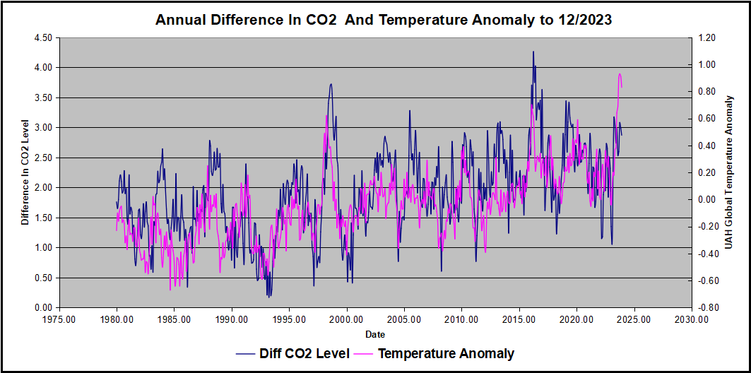
Here are UAH temperature anomalies compared to CO2 monthly changes year over year.

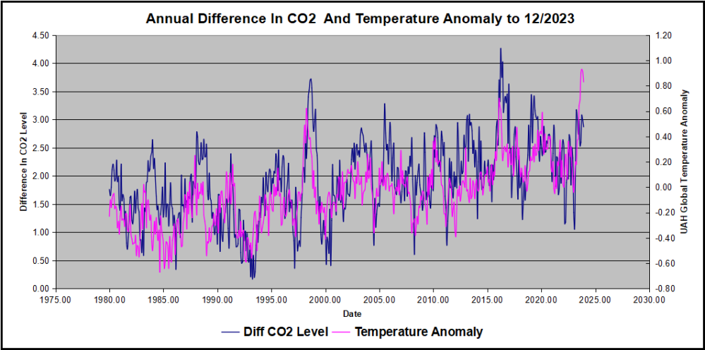
Changes in monthly CO2 synchronize with temperature fluctuations, which for UAH are anomalies now referenced to the 1991-2020 period. As stated above, CO2 differentials are calculated for the present month by subtracting the value for the same month in the previous year (for example June 2022 minus June 2021). Temp anomalies are calculated by comparing the present month with the baseline month.

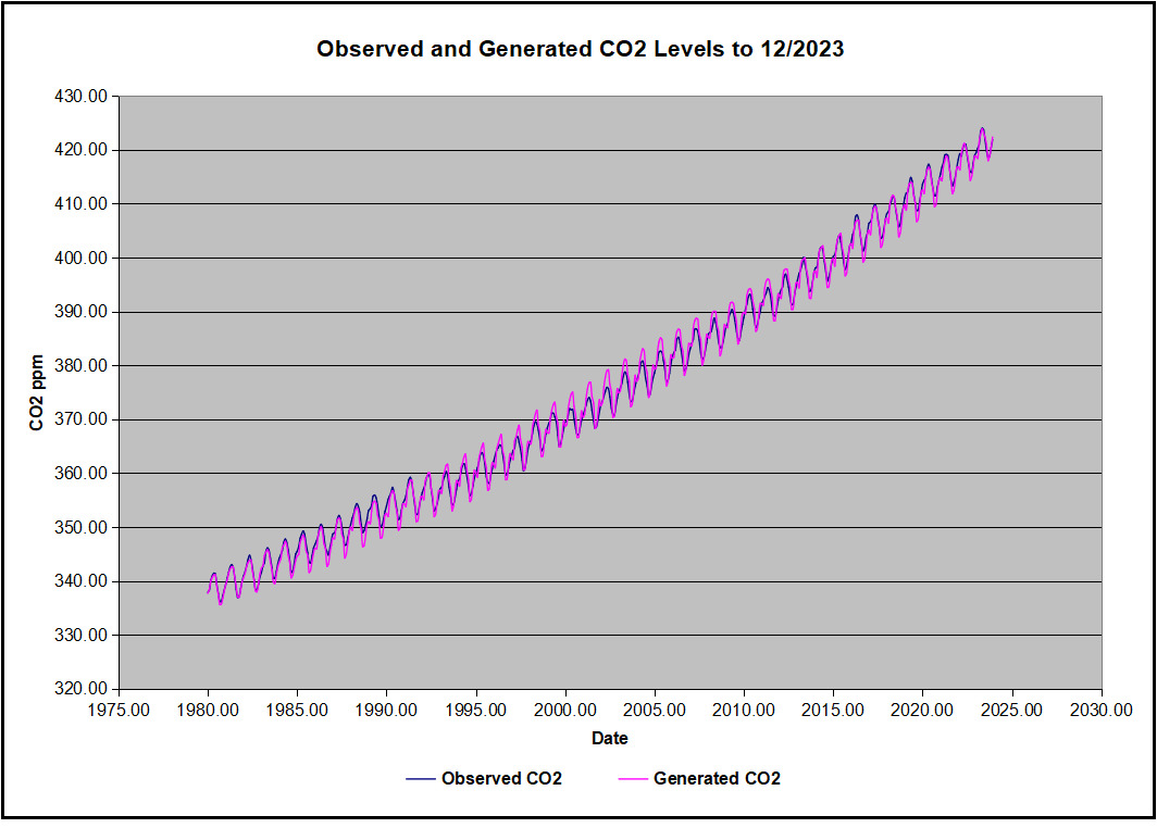
The final proof that CO2 follows temperature due to stimulation of natural CO2 reservoirs is demonstrated by the ability to calculate CO2 levels since 1979 with a simple mathematical formula:

For each subsequent year, the co2 level for each month was generated

CO2 _{this month this year} = a + b × Temp _{this month this year} + CO2 _{this month last year}

Jeremy used Python to estimate a and b, but I used his spreadsheet to guess values that place for comparison the observed and calculated CO2 levels on top of each other.

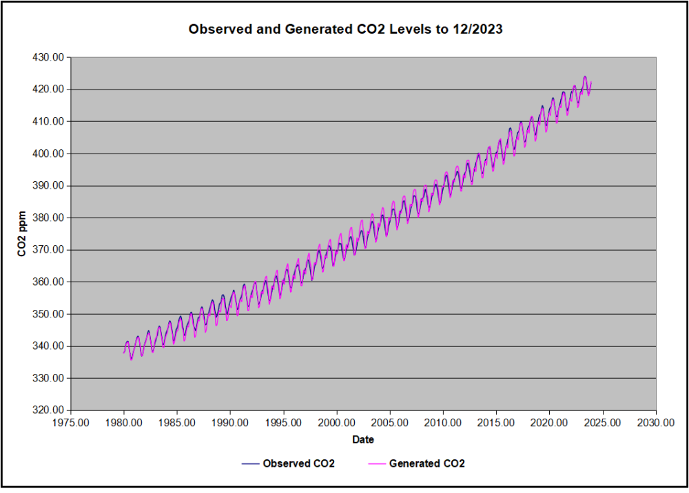
In the chart calculated CO2 levels correlate with observed CO2 levels at 0.9986 out of 1.0000. This mathematical generation of CO2 atmospheric levels is only possible if they are driven by temperature-dependent natural sources, and not by human emissions which are small in comparison, rise steadily and monotonically.

Comment: UAH dataset reported a sharp warming spike starting mid year, with causes speculated but not proven. In any case, that surprising peak has not yet driven CO2 higher, though it might, but only if it persists despite the likely cooling already under way.

Previous Post: What Causes Rising Atmospheric CO2?

nasa_carbon_cycle_2008-1

This post is prompted by a recent exchange with those reasserting the “consensus” view attributing all additional atmospheric CO2 to humans burning fossil fuels.

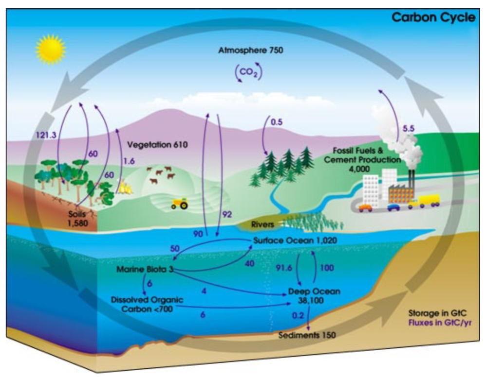
The IPCC doctrine which has long been promoted goes as follows. We have a number over here for monthly fossil fuel CO2 emissions, and a number over there for monthly atmospheric CO2. We don’t have good numbers for the rest of it-oceans, soils, biosphere–though rough estimates are orders of magnitude higher, dwarfing human CO2. So we ignore nature and assume it is always a sink, explaining the difference between the two numbers we do have. Easy peasy, science settled.

What about the fact that nature continues to absorb about half of human emissions, even while FF CO2 increased by 60% over the last 2 decades? What about the fact that in 2020 FF CO2 declined significantly with no discernable impact on rising atmospheric CO2?

These and other issues are raised by Murray Salby and others who conclude that it is not that simple, and the science is not settled. And so these dissenters must be cancelled lest the narrative be weakened.

The non-IPCC paradigm is that atmospheric CO2 levels are a function of two very different fluxes. FF CO2 changes rapidly and increases steadily, while Natural CO2 changes slowly over time, and fluctuates up and down from temperature changes. The implications are that human CO2 is a simple addition, while natural CO2 comes from the integral of previous fluctuations. Jeremy Shiers has a series of posts at his blog clarifying this paradigm. See Increasing CO2 Raises Global Temperature Or Does Increasing Temperature Raise CO2 Excerpts in italics with my bolds.

The following graph which shows the change in CO2 levels (rather than the levels directly) makes this much clearer.

Note the vertical scale refers to the first differential of the CO2 level not the level itself. The graph depicts that change rate in ppm per year.

There are big swings in the amount of CO2 emitted. Taking the mean as 1.6 ppmv/year (at a guess) there are +/- swings of around 1.2 nearly +/- 100%.

And, surprise surprise, the change in net emissions of CO2 is very strongly correlated with changes in global temperature.

This clearly indicates the net amount of CO2 emitted in any one year is directly linked to global mean temperature in that year.

For any given year the amount of CO2 in the atmosphere will be the sum of

all the net annual emissions of CO2
in all previous years.

For each year the net annual emission of CO2 is proportional to the annual global mean temperature.

This means the amount of CO2 in the atmosphere will be related to the sum of temperatures in previous years.

So CO2 levels are not directly related to the current temperature but the integral of temperature over previous years.

The following graph again shows observed levels of CO2 and global temperatures but also has calculated levels of CO2 based on sum of previous years temperatures (dotted blue line).

Summary:

The massive fluxes from natural sources dominate the flow of CO2 through the atmosphere. Human CO2 from burning fossil fuels is around 4% of the annual addition from all sources. Even if rising CO2 could cause rising temperatures (no evidence, only claims), reducing our emissions would have little impact.