This is the first of what will likely be a series of posts regarding urban heat island (UHI) effects in daily record high temperatures. My previous UHI work has been using the GHCN monthly average station data of “Tavg” (the average of the daily maximum [Tmax] and minimum [Tmin] temperatures). So, I’m moving from Tavg to Tmax (since record high temperatures are of so much interest), and daily rather than monthly values (although I will also sometimes include monthly results to provide context).
This post is mostly a teaser. Toward the end I will describe a new dimension to our UHI work I’m just starting.
The 2024 Poster Child for U.S. Warming: Palm Springs, CA
I was guided by a Google search on U.S. record high temperatures for 2024, and it seems Palm Springs, California was the place to start.
With a name like “Palm Springs” this place sounds like a wonderful spot to lounge under palm trees and enjoy the cool, refreshing spring water that surrounds you. Instead, the location is largely a desert, with the original downtown spring spitting out 26 gallons a minute of hot water. The “palms” do exist… they are “desert palms”, naturally growing in clusters where groundwater from mountain snowmelt seeps up through fissures connected to the San Andreas fault.
Like all U.S. metropolitan areas, the population growth at Palm Springs in the last 100+ years has been rapid. Even in the last 50 years the population has nearly doubled. Natural desert surfaces have been replaced with pavement and rooftops, which reach higher temperatures than the original desert soil, and the “impervious” nature of artificial surfaces (little air content) means the heat is conducted downward, leading to long-term storage of excess heat energy and, on average, higher temperatures. More on “impervious” surfaces later….
The Palm Springs Airport Weather Observation Site
The following Google Earth image shows the current location of the official ASOS (Automated Surface Observing System) site at the Palm Springs Airport, which recorded an all-time record high temperature of 124 deg. F on July 5 of this year.
What is somewhat amusing is that ASOS meteorological instrument siting guidance favors natural surfaces for placement, but since most of these weather stations are at airports (and since they primarily support aviation weather needs, not climate monitoring needs), the “natural” location is usually right next to runways, aircraft, and paved roads.
The next Google Earth image is zoomed out to show the greater Palm Springs area, with the ASOS site in the center (click on the image to zoom, then click to zoom more).
Record July Temperatures and Urbanization
It only makes sense that people want to know the temperature where they live, and most of the U.S. population resides in urban or suburban locations. Yet, the temperatures they experience are, probably without exception, higher than before people moved there and started building roads, buildings, and airports.
But what is misleading for those following the global warming narrative is that record high temperatures reported at these locations almost always mention climate change as a cause, yet they have no way of knowing how much urbanization has contributed to those record high temperatures. (Remember, even without global warming, high temperature records will continue to be broken as urbanization increases).
As mentioned above, on July 5, 2024 Palm Springs broke its all-time high temperature record, reaching 124 deg. F. There are 26 other daily GHCN stations within 40 miles of Palm Springs, all with varying levels of urbanization, but even more importantly, at very different elevations. If we plot the high temperatures reported for July 5 at those stations as a function of station elevation, we see that Palm Springs is an “outlier”, 5 degrees warmer than would be expected based upon its elevation-corrected expected temperature (the dashed regression line):
Now, keep in mind that many (if not most) of those 26 surrounding stations have their own levels of urbanization, making them hotter than they would be in the absence of pavement and roofs. So, that 5 deg. F excess is likely an underestimate of how much urban warming contributed to the Palm Springs record high temperature. Palm Springs was incorporated in 1938, and most population growth there has been since World War II.
If you are curious how the previous plot looks for the average of all July temperatures, here it is:
For the month of July, Palm Springs averaged 3 deg. F warmer than the surrounding stations (after adjusting for elevation effects, and keeping in mind that most of the *other* stations likely have their own levels of urbanization).
Clearly, Palm Springs has had spurious warming influence from the airport and surrounding urbanization which did not exist 100 years ago. But how much?
Impervious Surface Data as a Surrogate for Urbanization
This blog post is a prelude to a new project we’ve started where we will compare daily (as well and monthly) temperatures to a relatively new USGS dataset of yearly impervious surface coverage from 1985 to 2023, based upon Landsat data. I had previously experimented with a “Built Up” dataset based upon Landsat data, but it turns out that was just buildings. The “impervious surface” dataset is what I believe will have the greatest direct physical connection to what causes most UHI warming: roads, parking lots, roofs, etc. I think this will produce more accurate results (despite being only ~40 years in length) than my population density work (which is, we hope, close to being accepted for publication).
The post below updates the UAH record of air temperatures over land and ocean. Each month and year exposes again the growing disconnect between the real world and the Zero Carbon zealots. It is as though the anti-hydrocarbon band wagon hopes to drown out the data contradicting their justification for the Great Energy Transition. Yes, there was warming from an El Nino buildup coincidental with North Atlantic warming, but no basis to blame it on CO2.
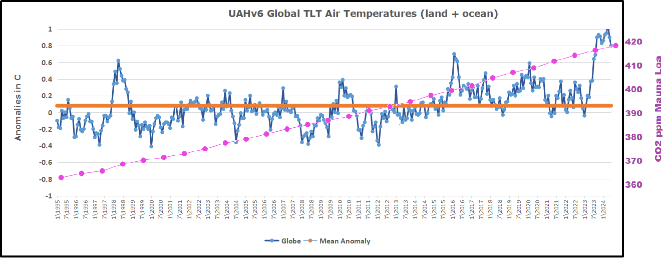
As an overview consider how recent rapid cooling completely overcame the warming from the last 3 El Ninos (1998, 2010 and 2016). The UAH record shows that the effects of the last one were gone as of April 2021, again in November 2021, and in February and June 2022 At year end 2022 and continuing into 2023 global temp anomaly matched or went lower than average since 1995, an ENSO neutral year. (UAH baseline is now 1991-2020). Now we have had an usual El Nino warming spike of uncertain cause, unrelated to steadily rising CO2 and now moderating.
For reference I added an overlay of CO2 annual concentrations as measured at Mauna Loa. While temperatures fluctuated up and down ending flat, CO2 went up steadily by ~60 ppm, a 15% increase.
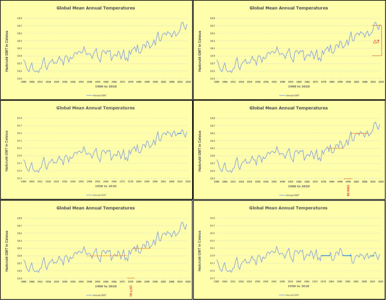
Furthermore, going back to previous warmings prior to the satellite record shows that the entire rise of 0.8C since 1947 is due to oceanic, not human activity.
The animation is an update of a previous analysis from Dr. Murry Salby. These graphs use Hadcrut4 and include the 2016 El Nino warming event. The exhibit shows since 1947 GMT warmed by 0.8 C, from 13.9 to 14.7, as estimated by Hadcrut4. This resulted from three natural warming events involving ocean cycles. The most recent rise 2013-16 lifted temperatures by 0.2C. Previously the 1997-98 El Nino produced a plateau increase of 0.4C. Before that, a rise from 1977-81 added 0.2C to start the warming since 1947.
Importantly, the theory of human-caused global warming asserts that increasing CO2 in the atmosphere changes the baseline and causes systemic warming in our climate. On the contrary, all of the warming since 1947 was episodic, coming from three brief events associated with oceanic cycles. And now in 2024 we have seen an amazing episode with a temperature spike driven by ocean air warming in all regions, along with rising NH land temperatures, now oscillating near its peak.
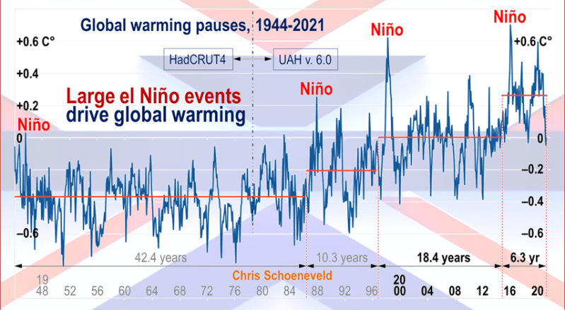
Chris Schoeneveld has produced a similar graph to the animation above, with a temperature series combining HadCRUT4 and UAH6. H/T WUWT
October 2024 Global Cooling Led by NH and Tropics Ocean and Land Temps
With apologies to Paul Revere, this post is on the lookout for cooler weather with an eye on both the Land and the Sea. While you heard a lot about 2020-21 temperatures matching 2016 as the highest ever, that spin ignores how fast the cooling set in. The UAH data analyzed below shows that warming from the last El Nino had fully dissipated with chilly temperatures in all regions. After a warming blip in 2022, land and ocean temps dropped again with 2023 starting below the mean since 1995. Spring and Summer 2023 saw a series of warmings, continuing into October, followed by cooling.
UAH has updated their TLT (temperatures in lower troposphere) dataset for October 2024. Due to one satellite drifting more than can be corrected, the dataset has been recalibrated and retitled as version 6.1 Graphs here contain this updated 6.1 data. Posts on their reading of ocean air temps this month are ahead of the update from HadSST4. I posted last month on SSTs using Ocean Cooling Resumes September 2024. These posts have a separate graph of land air temps because the comparisons and contrasts are interesting as we contemplate possible cooling in coming months and years.
Sometimes air temps over land diverge from ocean air changes. In July 2024 all oceans were unchanged except for Tropical warming, while all land regions rose slightly. In August we saw a warming leap in SH land, slight Land cooling elsewhere, a dip in Tropical Ocean temp and slightly elsewhere. September showed a dramatic drop in SH land, overcome by a greater NH land increase. Now in October, ocean and land temps in both NH and Tropics dropped, pulling the global anomaly down.
Note: UAH has shifted their baseline from 1981-2010 to 1991-2020 beginning with January 2021. v6.1 data was recalibrated also starting with 2021. In the charts below, the trends and fluctuations remain the same but the anomaly values changed with the baseline reference shift.
Presently sea surface temperatures (SST) are the best available indicator of heat content gained or lost from earth’s climate system. Enthalpy is the thermodynamic term for total heat content in a system, and humidity differences in air parcels affect enthalpy. Measuring water temperature directly avoids distorted impressions from air measurements. In addition, ocean covers 71% of the planet surface and thus dominates surface temperature estimates. Eventually we will likely have reliable means of recording water temperatures at depth.
Recently, Dr. Ole Humlum reported from his research that air temperatures lag 2-3 months behind changes in SST. Thus cooling oceans portend cooling land air temperatures to follow. He also observed that changes in CO2 atmospheric concentrations lag behind SST by 11-12 months. This latter point is addressed in a previous post Who to Blame for Rising CO2?
After a change in priorities, updates are now exclusive to HadSST4. For comparison we can also look at lower troposphere temperatures (TLT) from UAHv6.1 which are now posted for October. The temperature record is derived from microwave sounding units (MSU) on board satellites like the one pictured above. Recently there was a change in UAH processing of satellite drift corrections, including dropping one platform which can no longer be corrected. The graphs below are taken from the revised and current dataset.
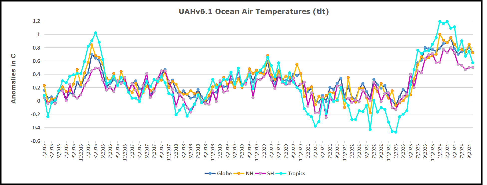
The UAH dataset includes temperature results for air above the oceans, and thus should be most comparable to the SSTs. There is the additional feature that ocean air temps avoid Urban Heat Islands (UHI). The graph below shows monthly anomalies for ocean air temps since January 2015.
In 2021-22, SH and NH showed spikes up and down while the Tropics cooled dramatically, with some ups and downs, but hitting a new low in January 2023. At that point all regions were more or less in negative territory.
After sharp cooling everywhere in January 2023, there was a remarkable spiking of Tropical ocean temps from -0.5C up to + 1.2C in January 2024. The rise was matched by other regions in 2024, such that the Global anomaly peaked at 0.95C in May, Since then the Tropics have cooled down to 0.6C, and the Global anomaly as well as NH dropped down to 0.7C in October.
Land Air Temperatures Tracking in Seesaw Pattern
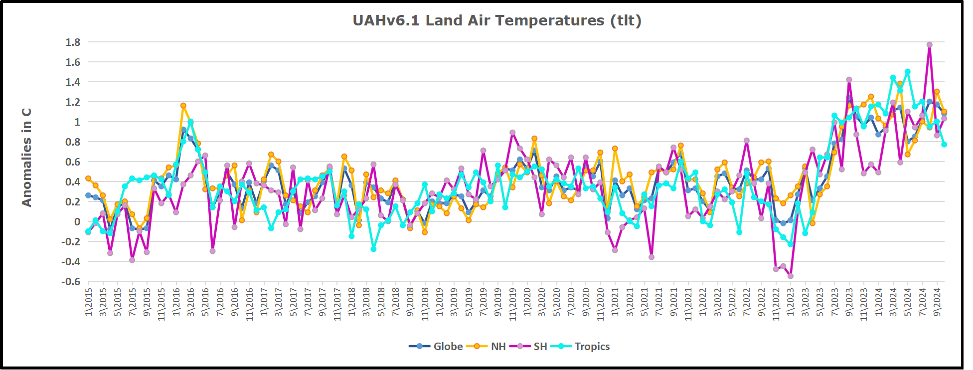
We sometimes overlook that in climate temperature records, while the oceans are measured directly with SSTs, land temps are measured only indirectly. The land temperature records at surface stations sample air temps at 2 meters above ground. UAH gives tlt anomalies for air over land separately from ocean air temps. The graph updated for October is below.
Here we have fresh evidence of the greater volatility of the Land temperatures, along with extraordinary departures by SH land. The seesaw pattern in Land temps is similar to ocean temps 2021-22, except that SH is the outlier, hitting bottom in January 2023. Then exceptionally SH goes from -0.6C up to 1.4C in September 2023 and 1.8C in August 2024, with a large drop in between. Now in October, NH and the Tropics have pulled the Global Land anomaly down despite a bump in SH land temps.
The Bigger Picture UAH Global Since 1980
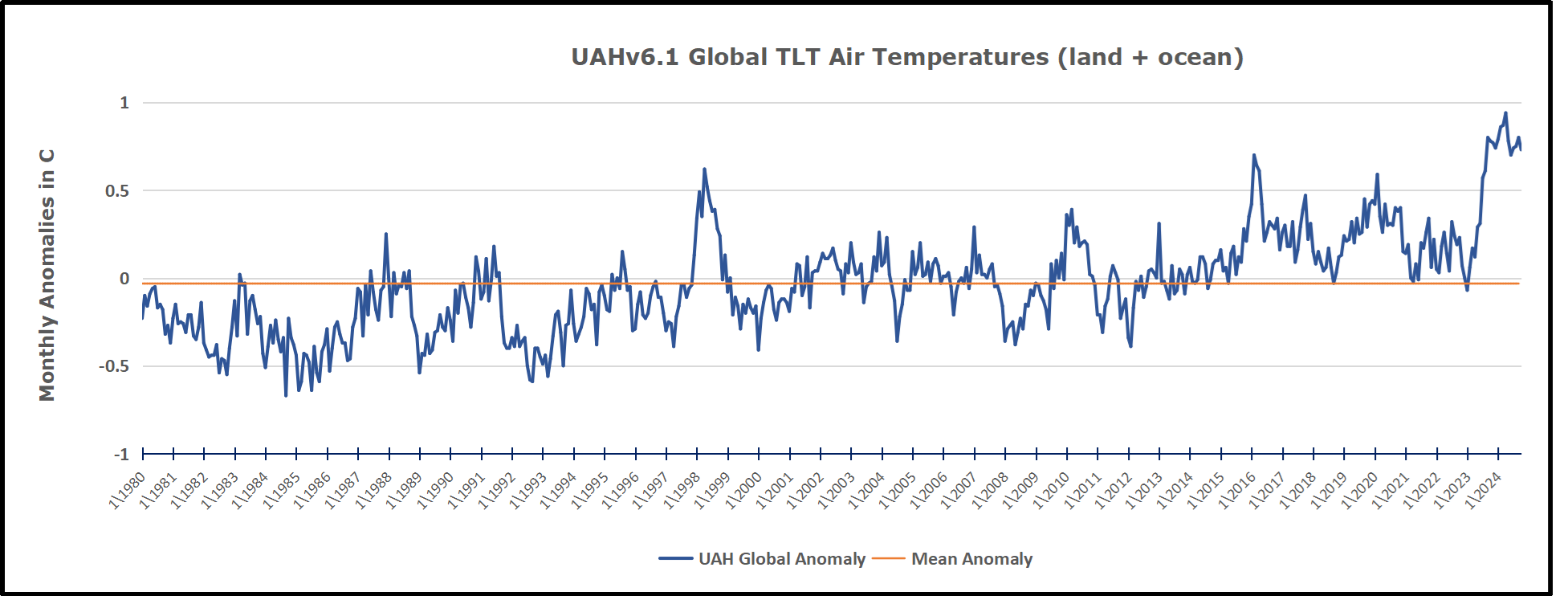
The chart shows monthly Global Land and Ocean anomalies starting 01/1980 to present. The average monthly anomaly is -0.03, for this period of more than four decades. The graph shows the 1998 El Nino after which the mean resumed, and again after the smaller 2010 event. The 2016 El Nino matched 1998 peak and in addition NH after effects lasted longer, followed by the NH warming 2019-20. An upward bump in 2021 was reversed with temps having returned close to the mean as of 2/2022. March and April brought warmer Global temps, later reversed
With the sharp drops in Nov., Dec. and January 2023 temps, there was no increase over 1980. Then in 2023 the buildup to the October/November peak exceeded the sharp April peak of the El Nino 1998 event. It also surpassed the February peak in 2016. In 2024 March and April took the Global anomaly to a new peak of 0.94C. The cool down started with May dropping to 0.90C, and in June a further decline to 0.80C. Now in October that temp is down to 0.7C.
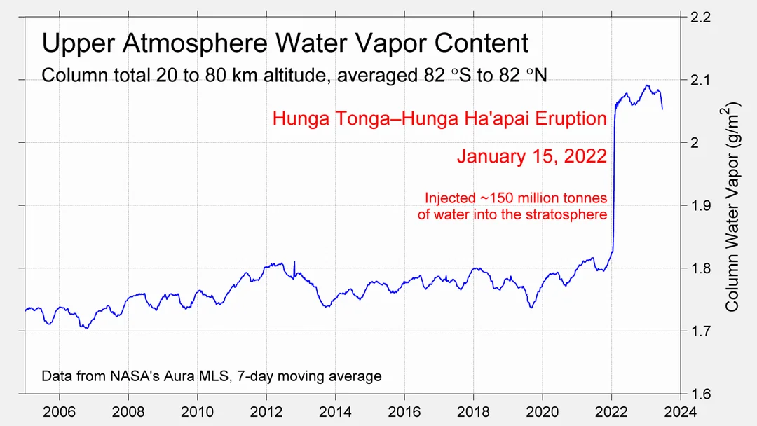
The graph reminds of another chart showing the abrupt ejection of humid air from Hunga Tonga eruption.
TLTs include mixing above the oceans and probably some influence from nearby more volatile land temps. Clearly NH and Global land temps have been dropping in a seesaw pattern, nearly 1C lower than the 2016 peak. Since the ocean has 1000 times the heat capacity as the atmosphere, that cooling is a significant driving force. TLT measures started the recent cooling later than SSTs from HadSST4, but are now showing the same pattern. Despite the three El Ninos, their warming had not persisted prior to 2023, and without them it would probably have cooled since 1995. Of course, the future has not yet been written.
“Consensus” scientists do not believe that solar variability, internal climate variability (in this model simplified to the ~67-year stadium wave), or volcanism influence net global warming or climate change since 1750, yet considerable evidence exists that these factors have an impact. I’ve previously built a model of the HadCRUT5 global average temperature (see here) from seven known climate and solar cycles using multiple regression and was reasonably successful.
In this attempt, I utilize the six best documented solar/climate cycles in listed Table 1 and the stadium wave climate-only interior variability cycle to create a multiple regression model of HadCRUT5.
Table 1. Solar and climate proxies and measurements used in this model.
When using many series to build a multiple regression model one is always confronted with von Neuman’s joke that with four arbitrary parameters he can fit an elephant. Further, all these series are serially correlated, which weakens the computed statistics of the resulting fit, such as R2. However, none of these series are “arbitrary parameters.” Except for the stadium wave and Log2_CO2 they are observed solar and climate cycles that share the same period and are in phase with one another. All are well supported with multiple lines of evidence. Thus, they are quite constrained and not arbitrary.
While they are not arbitrary in the von Neuman sense, they are not independent of one another. Probably the solar dynamo is behind all of them, but the mechanism Sun → climate is not understood for any of them except possibly for the Hale Cycle and the Barycenter. The solar dynamo is quite complex, especially in the longer term.
The stadium wave has no associated solar cycle and seems to be wholly internal variability, it has a period of roughly 67 years and correlates well with global average temperature (May & Crok, 2024). Internal climate variability is poorly understood and simply choosing the stadium wave to represent it is probably a vast oversimplification, but it is the best I can do. For a good up-to-date discussion of the components of internal variability I recommend Marcia Wyatt’s excellent report on circulation patterns (Wyatt M. , Circulation Patterns: Atmospheric and Oceanic, 2020). The report is paywalled, but a slightly different earlier version of the same report can be downloaded here.
The whole point of including the stadium wave is to account for the variable lag in emitting received solar radiation to space. Most solar radiation is received in the tropics, more than they can emit to space. As a result, some of the radiation received in the tropics must be transported to higher latitudes which emit more energy than they receive, especially in the winter months. Atmospheric and ocean circulation patterns change the timing of this tropics-to-pole energy transfer. A longer time to emit absorbed solar energy causes the planet to warm and a shorter time causes it to cool. Earth is never in thermal equilibrium except briefly by coincidence and the thermal energy residence time in the ocean/atmosphere climate system is constantly changing but seems to have roughly a 67-year cycle. The 67-year cycle overlies a longer secular trend of change, that longer trend could be due to solar cycles or CO2 or both. See figure 2 in May & Crok as an example.
There are no measurements from space or in the atmosphere that support the hypothesis that additional CO2 (man-made or otherwise) will cause global warming, but there are lab measurements, correlations, and climate models that support the hypothesis. CO2 has some effect, but how much is anyone’s guess at this point. We try and use multiple regression to derive a value below.
Critical Solar and Cycles
In this section we briefly describe each of the six well documented solar cycles listed in Table 1 that have a demonstrated impact on Earth’s climate and provide references for them.
Bray/Hallstatt Cycle
Roger Bray used glacial advance and retreat records to identify an approximately 2400-year climate cycle originally called the “Hallstatt” cycle (Bray, 1968). Although originally discovered by its effect on Earth’s climate there is an associated solar cycle that is in phase with the climate cycle and has the same period as discussed here. A more technical discussion of the solar Bray/Hallstatt Cycle is presented by Ilya Usoskin et al. here (Usoskin, Gallet, Lopes, Kovaltsov, & Hulot, 2016). A low in the Bray Cycle played a role in creating the very cold period from about 1650-1715AD during the Little Ice Age.
Eddy Cycle
The roughly 1000-year Eddy Cycle was named by José A. Abreu and colleagues (Abreu, Beer, & Ferriz-Mas, 2010). They note that John Eddy identified and documented periods of very low solar activity that corresponded with colder climates on Earth, like the Little Ice Age (Eddy, 1976). The 1000-year climate cycle can be seen by combining the Medieval Warm Period (roughly 800 to 1250AD with the Little Ice Age (roughly 1300-1850AD). Solar proxies find a 1000-year solar cycle that is in phase with the climate cycle as pointed out by John Eddy, see figure 5 in (Eddy, 1976). More on the Eddy Cycle can be seen in Javier Vinós’ book (Vinós, 2022), Chapter 8, page 123 here. The powerful Bray Cycle and the Eddy Cycle both had lows between 1470 and 1680 which undoubtably contributed to that extremely cold time during the Little Ice Age. For more on the Little Ice Age see (May & Crok, 2024) and here.
De Vries Cycle
The De Vries Cycle is also often called the Suess Cycle after Hans Suess (Suess, 1955) and (Sonett & Suess, 1984). Like most cycles it was first discovered in climate proxies, especially tree ring records, and it has a period of 193-209 years. The matching solar cycle is probably related to a beat period between the fundamental Hale Solar Cycle and the rosette-like motion of the Sun around the solar system barycenter (Stefani, Horstmann, Klevs, Mamatsashvili, & Weier, 2023).
Feynman Cycle
It was always recognized that some sort of solar cycle existed with a period between 50 and 150 years and the mysterious poorly defined cycle was usually called the Gleissberg Cycle. Meanwhile a climate cycle with a length of about 100 years was also observed. Eventually Joan Feynman nailed down what is now called the ~100-year Feynman Solar Cycle in 2014 (Vinós, 2022, p. 129) and (Feynman & Ruzmaikin, 2014). We use a period of 105 years for the Feynman Cycle. The Feynman climate and solar cycles have the same period and are in phase.
Hale Cycle
The 22.14-year Hale Cycle is a very prominent solar cycle that is formed by a 22-year fundamental period of solar magnetic activity. It encapsulates two solar cycles that are marked by reversals of the solar magnetic field. Thus, one Hale cycle sees a reversal of the magnetic field and then a return to the original polarity. The Hale Cycle is closely related to the 22-year southwestern U.S. drought cycle (Mitchell, Stockton, & Meko, 1979).
Solar Barycenter rosette
The Sun tracks a complicated rosette-like motion about the solar system barycenter that takes 19.86 years (Stefani, Horstmann, Klevs, Mamatsashvili, & Weier, 2023). Any climate cycle associated with this is buried, or possibly shared, with the Hale Cycle.
Other Natural Climate Cycles
Stadium Wave
What we call the Stadium Wave Cycle or oscillation is a very strong global climate cycle that has a period of about 67 years (Wyatt & Curry, Role for Eurasian Arctic shelf sea ice in a secularly varying hemispheric climate signal during the 20th century, 2014) and (Wyatt M. G., 2012c). It is composed of many climate oscillations that propagate in an organized fashion across the Northern Hemisphere and affect the climate of much of the globe. It is not clear if this oscillation is related to a solar cycle.
CO2
CO2 as a factor that influences climate was first properly described by Svante Arrhenius in his book Worlds in the Making (Arrhenius S. , 1908), but he also discusses it in an earlier paper (Arrhenius S. , 1896). Even before Arrhenius’ attempt to quantify the atmospheric CO2 concentration’s impact on the climate, the idea that CO2 can affect Earth’s climate was also discussed, although in a less quantitative way, by Fourier (Fourier, 1824), Tyndall (Tyndall J. , 1861) and (Tyndall J. , 1859), and Langley (Langley, 1884). None of these earlier writers suggested that atmospheric CO2 concentration “controlled the climate,” as the IPCC proposes in AR6 and previous reports (IPCC, 2021, p. 179), (Lacis, Hansen, Russell, Oinas, & Jonas, 2013), and (Lacis, Schmidt, Rind, & Ruedy, 2010). They also did not believe that human CO2 and other greenhouse gas emissions were responsible for almost all the warming Earth has experienced since 1750 as claimed by the IPCC in AR6, page 961, figure 7.7.
None-the-less, CO2 and other greenhouse gas concentrations probably do influence the average atmospheric temperature, however the idea that they somehow “control” the global average surface temperature and climate change is highly doubtful.
Figure 1 is a plot of all the series discussed in this post.
Figure 1. The time series discussed in this post.
Discussion
If we use the top seven series listed in table one, that is everything but CO2, and regress against HadCRUT5 we get the result shown in orange in figure 2. If we then regress everything, including CO2, we get the blue dashed line in figure 2. The two lines are nearly identical.
Figure 2. The faint gray line is HadCRUT5, the orange line is a regression against it using only the solar and climate cycles, the blue dashed line uses the same cycles, but adds the Log, base 2, of CO2.
Now, that is interesting! The fit with the climate/solar cycles only and the fit with CO2 and the same cycles are nearly identical. We need more information to make sense of this. Below are the statistics of the two regressions.
Table 2. Statistics of the regression with all the solar/climate cycles, but no CO2. Adjusted R2 = 0.8523.
Table 2 shows the statistics of the regression with no CO2. The derived coefficients are on the left, and the mean and standard deviation of each series are shown and then the normalized coefficients. We can see that the Bray and Eddy Cycles are the most important series, and they slightly oppose one another since they have different signs. All the “P” values are good. The standard errors for the Bray and Eddy Cycles are a bit high, but that may be because their coefficients have opposite signs.
In Table 3 we show the statistics for the regression that contains CO2.
Table 3. The regression statistics when CO2 is added. Adjusted R2 = 0.8548
Table 3 contains a lot of new and valuable information. In Table 2 the normalized coefficients show that the Bray and Eddy Cycles dominated the regression, but in Table 3 it is CO2, by a long way and the P values for both Bray and Eddy have become unacceptable. CO2 has essentially replaced the strong Bray and Eddy Cycles and knocked them out. Removing those two cycles results in the De Vries cycle becoming unacceptable with a P value of 0.37, so I also removed it, and the result is shown in Table 4.
Table 4. The regression statistics when CO2 is added. Adjusted R2 = 0.8548
In Table 4 all the P values are acceptable and CO2 dominates the regression. For all practical purposes the adjusted R2 from all three regressions are identical at about 0.85. The “adjusted R2” is corrected for the number of predictor variables and the number of observations. In all these cases the regular R2 is nearly identical to the adjusted R2.
Figure 3 compares the no CO2 case to the case described in Table 4.
Figure 3. Comparing the all-cycles/no CO2 regression in blue to the CO2 and no Bray, Eddy or de Vries cycles in orange. Statistics for the orange regression are given in Table 4.
Conclusions
As usual in climate science (and statistical analysis) you can take away whatever you like from this analysis. Statistics and climate science are similar in this way, you can always generate a lot of discussion around either of them and still know nothing.
CO2 makes no difference if all the climate/solar cycles are used, but CO2 can replace the most powerful Bray, Eddy, and de Vries solar/climate cycles. Objectively, one could point out that solar cycles (including the Milankovitch cycles) have driven climate change as far back as we can trace them with proxies and historical records, so why would we think CO2 is driving climate if adding it to the regression makes no difference?
On the other hand, CO2 can replace the very powerful Bray, Eddy, and de Vries cycles and get the same result. As usual, this analysis just shows we have no clue what drives climate change, but isn’t that what we’ve been saying all this time?
One can look at these plots and statistics and conclude that the impact of CO2 on climate is zero, or they can conclude it is 100%. This study is inconclusive by itself. However, it also shows that well-known solar cycles, combined with internal variability can explain recent global warming; CO2 is not required to explain it.
As with all purely statistical studies, this regression model is unsuitable to use in forecasting or hindcasting, the large coefficients in tables 2 to 4 show that. The value of the study is only to demonstrate that CO2 is not necessary to explain recent warming.
This post looks at the problem “does CO2 control global warming?” from a statistical perspective. To see how experts in climate science look at it from an atmospheric physics perspective it is worth reviewing the excellent 2014 American Physical Society workshop on climate change hosted by Steve Koonin. It is discussed and summarized here.
This post is the result of many email conversations with Charlie May, who contributed substantially to the ideas and models presented herein.
If Trump Is Elected It Will Be The End Of Bureaucracy As We Know It
Other Democrats agreed that another Trump presidency would likely spell doom for lucrative but wasteful government programs, with increased efficiency and reduced tax revenue taken in by the government would have a devastating effect on their ability to become wealthy. “Our system of government has never faced a more imminent threat,” said Congresswoman Nancy Pelosi. “The days of elected officials getting rich from kickbacks, secret bribes, and insider trading may be over. Serving the public should never be the motivating factor for entering public service. I fear for our nation… and my life.”
The gap between the media and the voters continues to grow:
Or, to put it another way, the media had to be nicer to Kamala than to any candidate in history
Newsbusters reports that this is the largest media bias they have ever seen. So despite the relentless propaganda, at least half the country know the media are barking mad, or they wouldn’t be doing the opposite to what the media wants them to do.
There is a citizens ECop group looking for help to archive election results in 15 minute intervals so audits can be done later. I can’t vouch for them, but it looks good. They aim to have a type of Election Results WayBack Machine. This would shine a light on any step-wise “jumps” in the vote tally.
Given Mike Benz withering description of 76 years of election rigging influence by US Intelligence agencies, it’s hard to believe they (and all the other beneficiaries) won’t be doing their damnedest to win one way or the other. After all their jobs may depend on it, and they’ve tried impeachment, indictments, assassinations, bankrupting him with legal cases, they’ve put his key supporters in jail, and they’ve disbarred the lawyers who tried to help him last time. What’s one more unthinkable steal? It’s just people protecting democracy.
Such is the weapons-grade demonization of Trump, Politico are having nightmares that Trump might lose and take power anyway. We all know they are just having wet dreams about what they want to do themselves. (Anything but respecting the will of the People.)
Activist groups have sprung up to defend the Blob
“The 65 Project” is a kind of legal Deathstar, threatening the lawyers who helped Donald Trump in 2020. They want to “deter future abuse of the legal system by “Big Lie Lawyers” (they actually call them that) seeking to overturn legitimate elections.” Legitimate, meaning, their favourite candidate.
Once upon a time, the opposition lawyers were just doing their job, but now they are are horrible unethical people who “risk democracy”presumably by bringing cases before the court that a judge might accidentally agree with. It’s so much more ethical to abandon the unwashed masses and deny them their day in court isn’t it?
It goes without saying that they must be afraid his lawyers might win.
Even if Trump is recognized as the winner, there are some plans to reject his electors on January 6
It isn’t over until the President is sworn in. Mike Benz talks about a group called The State Democracy Defenders Action — who want to kill democracy by crushing any attempts to question the official Blob declaration. This is the team that wants to use lawfare against Democracy Deniers.
Rep. Jamie Raskin (D) has said “it doesn’t matter who people vote for on November 5th”... Congress is going to not-certify the electoral college on January 6th, by citing Article 3 of the 14th Amendment. They will nullify him at the 11th hour, by saying Donald Trump is an insurrectionist.
See Just the News for more: In March the US Supreme Court overturned a Colorado effort to throw Trump off the ballot because he was a so-called “insurrectionist”. The Supreme Court ruled that only Congress could enforce the 14th Amendment, whereupon Jamie Raskin said they would revise their new legislation so they could get around the Supreme Court decision.
For any US voters reading, don’t forget to vote.
And while you wait, Joe Rogan talks to the most amazing engineer…
The more votes there are, the harder it is to sabotage.