Guest geology lesson by David Middleton

PETM = Paleocene-Eocene Thermal Maximum

Research Article
Temporal Scaling of Carbon Emission and Accumulation Rates: Modern Anthropogenic Emissions Compared to Estimates of PETM Onset Accumulation

Philip D. Gingerich
First published: 30 January 2019

[…]

Plain Language Summary
The Paleocene‐Eocene thermal maximum (PETM) is a global greenhouse warming event that happened 56 million years ago, causing extinction in the world’s oceans and accelerated evolution on the continents. It was caused by release of carbon dioxide and other greenhouse gases to the atmosphere. When we compare the rate of release of greenhouse gases today to the rate of accumulation during the PETM, we must compare the rates on a common time scale. Projection of modern rates to a PETM time scale is tightly constrained and shows that we are now emitting carbon some 9–10 times faster than during the PETM. If the present trend of increasing carbon emissions continues, we may see PETM‐magnitude extinction and accelerated evolution in as few as 140 years or about five human generations.

American Geohysterical Union

H/T to Jack Dale for this gem.

Gingerich, 2019 is a recent paper reiterating the PETM Chicken Little of the Sea meme. In the comments section of a recent post, it was cited as evidence of imminent catastrophe and followed up by a comment featuring this image from Clean Tecnica:

I just had to track this back to the Clean Tecnica article… Their scientific prowess is almost always laughable… And I was not disappointed.

Atmosphere Absorbing CO₂ Faster Than PETM, When Dinosaurs Perished

March 22nd, 2016 by Sandy Dechert

A new study in Nature Geoscience, led by Richard Zeebe of the University of Hawaii, looked at an anomalous time period called the Palaeocene-Eocene Thermal Maximum, or PETM. This phenomenon occurred about 56 million years ago, about ten million years following the beginning of the Cenozoic era (Age of Mammals), just about when the dinosaurs became extinct.

During the PETM, concentrations of carbon dioxide in the atmosphere spiked by 5 degrees Celsius, far higher than they have risen since human preindustrial levels 200 years ago. Climate scientists and world policy makers agree that 2 degrees more is all humans can probably take—or maybe 1.5, as more cautious voices are warning.

[…]

The investigation indicates that earth’s population now is emitting carbon into the atmosphere faster than carbonization at any other time in earth’s history since the PETM. Zeebe explains:

“If you look over the entire Cenozoic, the last 66 million years, the only event that we know of at the moment, that has a massive carbon release, and happens over a relatively short period of time, is the PETM. We actually have to go back to relatively old periods, because in the more recent past, we don’t see anything comparable to what humans are currently doing.”

In fact, our current rate of anthropogenic carbon release is at least an order of magnitude (10x) higher than what the world experienced during the PETM. The study concludes that “given that the current rate of carbon release is unprecedented throughout the Cenozoic, we have effectively entered an era of a no-analogue state.” In other words, earth has apparently never seen a situation like today’s for at least 66 million years, if ever. At that time, the hothouse world lasted over 1,000 centuries.

Clean Tecnica

What journalistic skills!

This phenomenon occurred about 56 million years ago, about ten million years following the beginning of the Cenozoic era (Age of Mammals), just about when the dinosaurs became extinct.

The PETM wasn’t “just about when the dinosaurs became extinct.”  10 million years later is not “just about when.” The K-T (or K-Pg) mass extinction wiped out 75% of all species on Earth, according to some estimates, taking out entire taxonomic genera and families, while putting serious dents into some orders and classes.

Apart from the mostly temporary extinction of some benthic foraminifera, the PETM was a period of thriving biodiversity.

This is one of the most priceless quotes ever…

During the PETM, concentrations of carbon dioxide in the atmosphere spiked by 5 degrees Celsius…

Zeebe et al., 2016 is actually a well-done bit of research, apart from the uber-alarmist title,  Anthropogenic carbon release rate unprecedented during the past 66 million years… Lions and tigers and bears!  Anthony covered it in this 2016 post here on WUWT.

Let’s just accept in arguendo that the modern rate of carbon release to the atmosphere and oceans is actually unprecedented in 66 million years… So what?

Almost all of the effect of CO₂ on temperature and seawater pH is essentially instantaneous.  The Transient Climate Response (TCR) is coincident with the rise in CO₂.  TCR is >80% of the total warming effect.  The remaining <20% occurs over hundreds of years, where it will be in the “noise level.”

Seawater pH is a function of Dissolved Inorganic Carbon (DIC, ΣCO₂) and Total Alkalinity (TA).

ΣCO₂ (DIC) and TA are “conservative quantities,” unaffected by changes in pressure and temperature and can be calculated if any two of two of the following parameters: pCO₂, pH (not pH) and ΣCO₂, and the total dissolved boron are known.

ΣCO₂ = [CO₂]+[HCO₃^–]+[CO₃^2-]

TA = [HCO₃^–]+ 2[CO₃^2-]+[B(OH)₄^–]+[OH^–]-[H⁺]

This process is also basically instantaneous.

A study of seawater pH near active volcanic CO₂ vents in the Mediterranean (Kerrison et al., 2011) found that the pH immediately adjacent to the vent was still alkaline, despite being subjected to the equivalent of nearly 5,600 ppm CO₂.

Partial pressure and fugacity (μatm) are a little lower than what the mixing ratio (ppm) would be, depending on temperature and humidity.  However, they are close.  A partial pressure (pCO₂) of 350 μatm generally equates to about 350 ppm in the atmosphere.   At nearly 5,600 ppm CO₂ the seawater was still alkaline, not acidic.

Even if anthropogenic carbon emissions are “unprecedented during the past 66 million years,” it’s clear that comparisons to the PETM are, at best, irrelevant and, at worst, intentionally misleading.

Our “unprecedented” carbon emissions will probably push atmospheric CO₂ to anywhere from 500 to 700 ppm by the end of this century.  Based on a real world “business as usual” emissions scenario, with oil consumption peaking around 2060, coal consumption remaining relatively stable, natural gas displacing oil at its current pace and no carbon tax, I come up with a CO₂ level right about inline with RCP 6.0, “a mitigation scenario, meaning it includes explicit steps to combat greenhouse gas emissions (in this case, through a carbon tax)“.

A realistic TCR of 1.5 °C per doubling of CO₂ yields about 2 °C of warming at 700 ppm, half of which has already occurred.

Contrasting the “Anthropocene” (fake word) with the PETM (real acronym)

The PETM was probably related to the formation of the North Atlantic Large Igneous Province (Storey et, al 2007), a period of intense volcanic activity associated with the opening of the North Atlantic Ocean.

PETM atmospheric CO₂ could have been anywhere from 400-800 to over 3,000 ppm.  The Mauna Loa CO₂ time series (MLO) doesn’t even break out of the Neogene noise level.

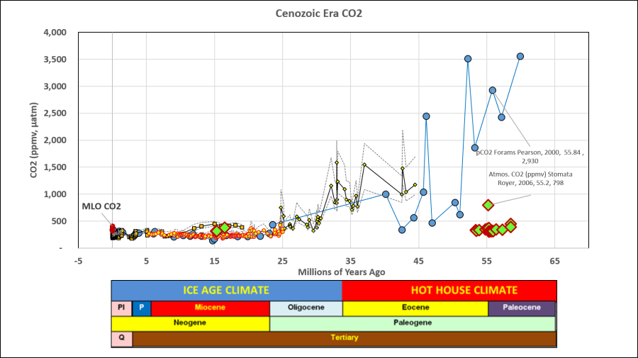
Note how the PETM (55 Ma) is about as far from a CO₂ analog to modern times as it possibly could be… unless the PETM stomata data are correct, in which case AGW is even more insignificant than previously thought.

Regarding temperatures, the PETM is also about as far from being an analog to modern times as it possibly could be.

Note that the Early Eocene Climatic Optimum (EECO) was just as warm as the PETM and lasted longer.

To demonstrate how utterly ridiculous it is to describe the PETM as an analog for modern climate change, we just have to look at the Miocene Epoch, which was much cooler than the PETM and EECO.

Bear in mind that the HadSST3 data are of much higher resolution than the δ¹⁸O time series.  The amplitude of the proxy time series on multi-decadal to centennial time-scales should be considered to be the minimum of the true variability on those time-scales, due to the much lower resolution than the instrumental data (Ljungqvist, F.C. 2010).  Despite this, the modern ~1 °C rise since pre-industrial times doesn’t even break out of the Pleistocene noise level… another 1 °C rise won’t even break out of the Pleistocene noise level.

The PETM is also often cited as an analog for Chicken Little of the Sea…

There simply is no analogy.  The paleogeography of the Cretaceous through the Eocene “Hot House Climate” was very different than the “Ice Age Climate” since the early Oligocene.   The warmth of the  PETM was mostly a function of plate tectonics.

The phrase “ocean acidification” was literally invented out of thin air in 2003 by Ken Caldiera.  The relationship between CO₂, DIC, TA and the distribution of pelagic sediments has been understood for a long time.

When the pH of seawater decreases, calcium carbonate dissolves.  In warm, shallow seas, at a pH of about 8.3, dissolution of aragonite and calcite particles by inorganic processes is almost nonexistent.  However, since the classical studies of the Challenger expedition, it has been known that the proportion of calcium-carbonate particles in seafloor sediments decreases as depth of water increases (Table 5-1).  Such decrease is particularly rapid at depths between 4000 and 6000 m.  Although the reasons for this decrease have been debated, the evidence suggests that calcium carbonate dissolves because the CO₂ concentration increases with depth.  The control on CO₂ appears to be part biological; it results from biological oxidation of organic-carbon compounds.  Also, the water masses at greater depth were derived from the polar region; their temperature is lower and the water contains more dissolved CO₂. Increased concentration of CO₂ is in turn reflected by lower pH, which leads to calcium carbonate dissolution.  However, the increase of pressure with depth may also be involved; such increase affects the dissociation of carbonic acid (Eqs. 5-11 and 5-12).  The depth at which the calcium-carbonate decreases most rapidly is known as the carbonate-compensation depth, defined as the depth at which the rate of dissolution of solid calcium carbonate equals the rate of supply.

Friedman and Sanders, pages 133-134. (1978)

Prior to Chicken Little of the Sea, the phrase was “shoaling of the lysocline” (a shallowing of the carbonate or calcite compensation depth).

The PETM exhibited a genuine shoaling of the lysoline.

During Ocean Drilling Program Leg 208, six sites were drilled at water depths between 2500 and 4770 m to recover lower Cenozoic sediments on the northeastern flank of Walvis Ridge. Previous drilling in this region (Deep Sea Drilling Project [DSDP] Leg 74) recovered pelagic oozes and chalk spanning the Cretaceous/Paleogene (K/P), Paleocene/Eocene, and Eocene/Oligocene boundaries. The objective of Leg 208 was to recover intact composite sequences of these “critical” transitions from a wide range of depths. Multichannel seismic data (Meteor Cruise M49/1) along with information from DSDP Leg 74 sites were used to identify sites where continuous sequences of lower Cenozoic sediment should be present. Double to triple advanced piston coring, occasional extended core barrel coring to deepen the holes, and high-resolution physical property measurements were employed to construct “composite sections.” The composite sections provide a detailed history of paleoceanographic variation associated with several prominent episodes of early Cenozoic climate change, including the K/P boundary, the Paleocene/Eocene Thermal Maximum (PETM), the early Eocene Climatic Optimum, and the early Oligocene Glacial Maximum.

The PETM interval, the main focus of Leg 208, was recovered at five sites along a depth transect of 2.2 km. The sediment sequence is marked by a red clay layer, which varies in thickness from 20 to 50 cm from site to site, within a thick and uniform sequence of upper Paleocene and lower Eocene foraminifer-bearing nannofossil ooze. The basal color contact is relatively sharp, although magnetic susceptibility data show a more gradual, steplike transition at the deeper Sites 1262 and 1267. The carbonate content drops to 0 wt% at all sites except for Site 1265. The upper contact is gradational in the shallow sites and relatively sharp at the deeper sites. Overlying the clay layer is a sequence of nannofossil ooze, which is slightly richer in carbonate than the unit immediately underlying the clay layer.

The depth transect permits testing of the leading hypothesis for the cause of the PETM: the abrupt dissociation of as much as 2000 Gt of marine methane hydrate. Numerical modeling demonstrates that the injection of such a large mass of carbon to the ocean/atmosphere could have triggered a rapid (~10 k.y.) global shoaling of the calcite compensation depth (CCD) and lysocline, followed by a gradual recovery, and “overcompensation” with the CCD overshooting pre-excursion depths. Based on sediment cores recovered during Leg 208, the CCD shoaled by >2 km during the excursion, considerably more than predicted in present carbon cycle models of the event.

Leg 208 material also documents biotic responses to environmental changes as a result of the methane release and CCD shoaling (e.g., severe dissolution over such a large depth range may well have been an important factor in the benthic foraminiferal extinction event coincident with the base of the clay layer at every site, and nannofossils showed a short-term relative abundance response from Fasciculithus to Zygrhablithus). Planktonic foraminifers are heavily dissolved in the clay layer with only extremely rare specimens of acarinids and morozovellids remaining.

The Leg 208 transect complements a transect drilled on the southern Shatsky Rise during Leg 198, a deep latitudinal transect in the equatorial Pacific drilled during Leg 199, a shallow to bathyal transect drilled on Demarera Rise during Leg 207, and a depth transect proposed for future drilling in the western North Atlantic Ocean (J-Anomaly Ridge and southeast Newfoundland Rise).

ODP Leg 208 Summary

The shoaling of the lysocline during the PETM is represented by the 30 cm thick band of red clay from 13.4 to 13.7 m on the lithology column in figure 15.  When the lysocline and carbonate compensation depth (CCD)  briefly shoaled, the transition from calcareous to siliceous ooze moved shoreward.  When the CCD dropped back down to its pre-PETM depth, the transition from calcareous to siliceous ooze moved seaward… Leaving a 30 cm thick layer of red clay in the middle of a thick marl sequence.  Rising and falling sea level could have left a similar layer of red clay.

The benthic foram’s above and below the red clay horizon ceased to exist at that location for about 70,000 to 220,000 years.  However, the fact that at least some of them returned to that location after the PETM might indicate that the benthic foram “mass extinction” was more of a benthic foram depositional “mass relocation,” rather than a true extinction.

The PETM lysocline shoaled by more than 2,000 m at Walvis Ridge… This is literally written in stone.

Over the past 250 years, since the beginning of the industrial revolution, there has been about a 16% decrease in aragonite and calcite saturation state in the Pacific Ocean. From repeat oceanographic surveys, we have observed an average 0.34% yr⁻¹ decrease in the saturation state of surface seawater with respect to aragonite and calcite over a 14‐year period. This has caused an upward migration of the aragonite and calcite saturation horizons toward the ocean surface on the order of 1–2 m yr⁻¹. These changes are the result of the uptake of anthropogenic CO₂ by the oceans, as well as other smaller scale regional changes in circulation over decadal time scales. If CO₂ emissions continue as projected out to the end this century, the resulting changes in the marine carbonate system would mean that many coral reef systems in the Pacific would probably no longer be able to maintain the necessary rate of calcification required to sustain their vitality.

Feely et al., 2012

The 16% decrease in aragonite and calcite saturation state in the Pacific Ocean over the past 250 years is entirely based on calculating the preindustrial aragonite and calcite from the assumed preindustrial atmospheric CO₂ concentration.  It is circular reasoning.  Regarding the claim that they’ve measured 14-28 m of shoaling over a 14-year period… That’s not even the margin of error in estimating the CCD. A genuine shoaling of the lysocline would cause a redistribution of pelagic (open ocean seafloor) sediments.

I have not been able to locate a more recent version of this map:

DISTRIBUTION OF PELAGIC SEDIMENTS
General Features of Distribution. Figure 253 shows the distribution of the various types of pelagic sediments. The representation is generalized partly to avoid confusion and partly because of the incomplete knowledge as to the types of sediments found in many parts of the oceans. Any such presentations of the distribution of pelagic sediments are modified versions of maps originally prepared by Sir John Murray and his associates. Further investigations have changed the boundaries but have not materially affected the general picture. The figure has been prepared from the most recent sources available. The distribution of sediments in the Indian Ocean is based on a map by W. Schott (1939a), that in the Pacific Ocean is from W. Schott in G. Schott (1935), with some revisions based on Revelle’s studies of the samples collected by the Carnegie (Revelle, 1936). The data for the Atlantic have been drawn from a number of sources, since no comprehensive map has been prepared for many years. The Meteormaterial has been described by Correns (1937 and 1939) and Pratje (1939a). Thorp’s report (1931) on the sediments of the Caribbean and the western North Atlantic was used for those areas, and Pratje’s data (1939b) for the South Atlantic were supplemented by those of Neaverson (1934) for the Discovery samples. The distribution in the North Atlantic is from Murray (Murray and Hjort, 1912).

One type of shading has been used for all of the calcareous sediments and another for the siliceous sediments. Unless the symbol P is shown to indicate that the area is covered with pteropod ooze, it is to be understood that the calcareous sediment is globigerina ooze. The siliceous organic sediments are indicated as D for diatom ooze and Rfor radiolarian ooze. The unshaded areas of the oceans and seas are covered with terrigenous sediments.

[…]

Sverdrup, Johnson & Fleming, 1942

The PETM resulted in a major redistribution of pelagic sediments. If Chicken Little of the Sea is like the PETM, the seafloor would exhibit a significant redistribution of pelagic sediments relative to 1942. More of the seafloor would be covered with siliceous ooze and far less would be covered by calcareous ooze. If anyone is aware of a recent map, like the one in my marine science text book, please let me know.

References

Colosimo, A.B, Bralower, T.J., and Zachos, J.C., 2006. “Evidence for
lysocline shoaling at the Paleocene/Eocene Thermal Maximum on Shatsky
Rise, northwest Pacific”. In Bralower, T.J., Premoli Silva, I., and Malone, M.J. (Eds.), Proc. ODP, Sci. Results, 198, 1–36

Dore, J.E., Lukas R., Sadler, D.W. Church, M.J., Karl, D.M. (2009).  “Physical and biogeochemical modulation of ocean acidification in the central North Pacific.” Proc Natl Acad Sci USA 106:12235–12240.

Friedman, G.M. and Sanders, J.E. (1978) “Principles of Sedimentology”. Wiley, New York.

Gingerich, Philip. (2019). “Temporal Scaling of Carbon Emission and Accumulation Rates: Modern Anthropogenic Emissions Compared to Estimates of PETM-Onset Accumulation”. Paleoceanography and Paleoclimatology. 10.1029/2018PA003379.  Abstract only.

Hoorn, C., Wesselingh, F.P., ter Steege, H.; Bermudez, M.A., Mora, A., Sevink, J., Sanmartin, I., Sanchez-Meseguer, A., Anderson, C.L., Figueiredo, J.P., et al. “Amazonian through time: Andean uplift,climate change, landscape evolution and biodiversity”. Science 2010, 330, 927–931

Kerrison, Phil & Hall-Spencer, Jason & Suggett, David & Hepburn, Leanne & Steinke, Michael. (2011). “Assessment of pH variability at a coastal CO2 vent for ocean acidification studies.” Estuarine and Coastal Marine Science. 94. 129-137. 10.1016/j.ecss.2011.05.025.

Pagani, M., J.C. Zachos, K.H. Freeman, B. Tipple, and S. Bohaty. 2005. “Marked Decline in Atmospheric Carbon Dioxide Concentrations During the Paleogene”. Science, Vol. 309, pp. 600-603, 22 July 2005.

Pearson, P. N. and Palmer, M. R.: Atmospheric carbon dioxide concentrations over the past 60 million years, Nature, 406, 695–699,https://doi.org/10.1038/35021000, 2000.

Royer, et al., 2001. Paleobotanical Evidence for Near Present-Day Levels of Atmospheric CO₂ During Part of the Tertiary. Science 22 June 2001: 2310-2313. DOI:10.112

Storey, Michael, Robert A. Duncan, Carl C Swisher 2007. “Paleocene-Eocene Thermal Maximum and the Opening of the Northeast Atlantic”. Science 27 April 2007: 587-589. DOI:10.1126

Sverdrup, H. U. M. W., Johnson and R. H. Fleming, “The Oceans—Their Physics, Chemistry, and General Biology,” Prentice-Hall, Upper Saddle River, 1942.

Tripati, A.K., C.D. Roberts, and R.A. Eagle. 2009.  “Coupling of CO₂ and Ice Sheet Stability Over Major Climate Transitions of the Last 20 Million Years”.  Science, Vol. 326, pp. 1394 1397, 4 December 2009.  DOI: 10.1126/science.1178296

Zachos, J. C., Pagani, M., Sloan, L. C., Thomas, E. & Billups, K. “Trends, rhythms, and aberrations in global climate 65 Ma to present”. Science 292, 686–-693 (2001).

Zachos, J.C., Kroon, D., Blum, P., et al., 2004. Proc. ODP, Init. Repts., 208: College Station, TX (Ocean Drilling Program). doi:10.2973/odp.proc.ir.208.2004

Zachos, et al., 2005. “Rapid Acidification of the Ocean During the Paleocene-Eocene Thermal Maximum”. Science 10 June 2005: 1611-1615. DOI:10.1126

Zeebe, R. E., A. Ridgwell, and J. C. Zachos (2016), “Anthropogenic carbon release rate unprecedented during the past 66 million years”.  Nat. Geosci., 9(4), 325–329, doi:10.1038/ngeo2681.

Zeebe, Richard E. and Dieter A. Wolf-Gladrow CARBON DIOXIDE, DISSOLVED (OCEAN)

Watts Up With That? Chicken Little of the Sea/PETM posts by David Middleton

Ocean Acidification: Chicken Little of the Sea Strikes Again

Chicken Little of the Sea Visits Station ALOHA

The Total Myth of Ocean Acidification

The Total Myth of Ocean Acidification, Part Deux: The Scientific Basis

Chicken Little of the Sea Is Dissolving the Sea Floor!!! Run Away!!!

New Paper: PETM Was Caused by Climate Change… Ancient Climate Change Caused Climate Change… AEUHHH????