Guest post by Nick Stokes,

People outside climate science seem drawn to feedback analogies for climate behaviour. Climate scientists sometimes make use of them too, although they are not part of GCMs. But it gets tangled. In fact, all that the feedback talk is usually doing is describing the behaviour of variables that satisfy a few linear equations. Feedback talk adds a way of thinking about this, but does not change the mathematics of linear equations.

A couple of articles I’ll refer to are a survey article by Roe, and a frequently cited 2006 article by Soden and Held.

The basic calculus behind feedback and linear signal analysis goes like this. You have a device or system with a number of state variables, which I’ll bundle into a vector x. And the physics requires that they satisfy a set of equations that I’ll write just as

f(x)=0
There is a particular set of values x₀ which satisfy those equations that for an amplifier, say, would be called the operating point. Generally it is a state existing prior to perturbation by an amount dx (a vector of state changes). After perturbation it still has to satisfy the equations, so

f(x₀)=0 and f(x₀+dx)=0

For linear amplifiers, the perturbed state can be well approximated by the derivative expression

f(x₀+dx) = f(x₀)+f'(x₀) dx = 0
and since f(x₀) = 0, that leaves the set of linear equations in the perturbation

f'(x₀) dx = 0
We don’t have to worry too much about the form of f'(x₀), or indeed f(x₀). The point is that it is linear, so all terms are proportional to perturbation. We can just take it that f'(x₀) is a matrix operating on the vector of perturbations dx. Roe (p 99) has a section headed “Feedbacks Are Just Taylor Series in Disguise”. Actually “Taylor Series” overstates it, since only first order terms are used. But it is getting close to the correct treatment as linear equations of perturbations.

Usually we think of one of the components of dx as the input, or forcing, and another as the output. Then the equations can be shaken down to make output proportional to input, or gain. This is just a property of a linear system of n equations in n+1 variables, and the feedback algebra just expresses it. But you don’t have to think of it that way. I’ll give some examples leading up to climate.

One thing that is important is that you keep the sets of variables separate. The components of x₀ satisfy a state equation. The perturbation components satisfy equations, but are proportional to the perturbation. You can’t mix them. This is the basic flaw in Lord Monckton’s recent paper.

Example 1 – the abstract feedback system

The Wiki description is as good as any. It’s labelled negative feedback, but applies generally. The diagram is:

with the accompanying text

Note that it starts with two equations in three unknown voltages. Two are overall input and output, and the third, V’, is the voltage at the input to the amplifier (triangle). V’ is eliminated, leading to an equation relating input and output (red star). This is then manipulated to a gain ratio. But all these steps are just standard high-school manipulations; they don’t add anything. A computer (or a student?) could have solved them at any stage.

Example 2 – a junction transistor

Here is a very simplified AC circuit, with bias arrangements and capacitors omitted. The voltages are the perturbations (AC). Simplified transistor properties are assumed – zero input impedance, infinite output, and a current amplification β=100. So the AC voltage at the base (V’) is held to zero. There are 3 unmarked currents, denoted by the suffices of the resistors I₀, I₁, I_f. Directions are I₀ right, I₁ down, I_f right. 5 variables in all.

So we write down linear relations. There are 3 Ohm’s Law

Vin=I0*R0

Vout=-I1*R1

Vout= -If*Rf

and one current gain relation:

β*(I₀ – I_f) = I₁ + I_f

Again, anything further done with these equations is just high school manipulation. But it can be shaken down to a voltage gain by eliminating currents, written in gain/feedback style:

V₁ = -β (R₁/R₀) V₀ / ( 1 + f) where f=(β+1)R₁/R_f

Note that it is an inverting amplifier, and the feedback is negative.

Example 3 – Climate feedbacks

Again, it’s just a matter of writing down linear equations, resulting here from equilibrium flux balance. I’ll follow this 2006 article of Soden and Held. Unfortunately, they don’t actually quite write the flux equations, but I’ll do it for them. They write:

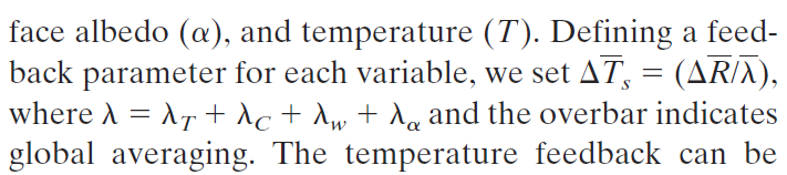
ΔR is the change in flux at TOA, which is the GHG forcing. ΔT is the surface temperature response. The feedback factors are T for temperature,w water vapor, C clouds and α (=a) for albedo. What they are actually doing (multiply by λ) is writing a flux balance

ΔR = λ_TΔT + λ_wΔT + λ_CΔT + λ_aΔT

Each term on the right represents a flux due to that factor. They do a bit extra, which I won’t go into, to deal with the fact that flux is at TOA and response is at surface. Their T flux is what people often call the Planck feedback; they roll into it other kinds of temperature dependent cooling, but it is mainly radiation (Stefan-Boltzmann etc).

This hopefully demystifies all the stuff about positive, negative feedback and runaway. The first is a big term that determines what is thought of as feedback-free (open-loop) gain. It is the 3.2 W/m^2/K figure that is often quoted, and turns into the 1.05K/doubling which forms the basis for Lord Monckton’s ECS. That comes from this paper. The other terms are mostly negative, so they diminish the coefficient of ΔT and so increase the amount ΔT must respond to stay in balance. That is interpreted as positive feedback.

It actually gives a perhaps less scary picture of thermal runaway. If these negative fluxes increase, there will come a point where the coefficient of ΔT is zero. That doesn’t mean instant flames. It just means there is nothing to counter heat accumulation from the forcing flux. So the temperature will indeed rise without limit (until some nonlinearity intervenes), but only as forced by the few W/m2 of ΔR. Not good, but not perhaps as dramatic as imagined. If the coefficient became negative, then there could be exponential rise, which might get more dramatic.

So did climatology make a startling error in omitting “reference temperature”.

I may have given away the answer, but anyway, it is, no! Soden and Held is a typical exposition. They correctly gather the perturbation terms – that is, the forcing, in terms of GHG heat flux, and the proportional responses. It is wrong to include variables from the original state equation. One reason is that the have been accounted for already in the balance of the state before perturbation. They don’t need to be balanced again. The other is that they aren’t proportional to the perturbation, so the results would make no sense. In the limit of small perturbation, you still have a big reference temperature term that won’t go away. No balance could be achieved.

So are all sets of linear equations to be regarded as amplification/feedback?

Well, nothing really hangs on it except the way you talk about them; the algebra is the same. But what characterises amplification is that one of the coefficients is large relative to the others. That means that changing that variable induces a large response in others (hence amplified). What is characterised as feedback is where this variable appears in at least one other term, and is also multiplied by the big coefficient. That makes a big proportional change in the output variables. That modifies the apparent performance in ways described as feedback.

So what is the outcome here? Mainly that you can talk about feedback, signals, Bode etc if you find it helps. But the underlying maths is just linear algebra, and the key thing is to write down correct perturbation equations, and manipulate them algebraically if you really want to. Or just solve them as they are.