This recent study (h/t to Jim Simpson) comes from Australia and was published in late 2019. It studies the impacts of global warming on the U.S. economy. What the authors have done is used one the climate models (the FUND model) to look ahead at the impacts warming would have on other economic sectors besides energy. Now that the “worst-case scenario” RCP8.5 model has been put out of favor by a recent paper, the 3.0°C warming scenario they used is more in-line with the RCP6 and RCP 4.5 models that remain. The work replicates and improves upon earlier work done by Dr. Richard Tol in 2009 in The Economic Effects of Climate Change.
What they found is surprising; the overall economic impact of 3.0°C global warming would be beneficial nor just for the United States, but the entire global economy.
They write in the introduction:
There is a scientific hypothesis and political acceptance that global warming of 2 °C or more above pre-industrial times would have a negative impact on global economic growth. This hypothesis is supported by economic models that rely on impact functions and many assumptions. However, the data needed to calibrate the impact functions is sparse, and the uncertainties in the modelling results are large. The negative overall impact projected by at least one of the main models, Climate Framework for Uncertainty, Negotiation and Distribution (FUND), is mostly due to one impact sector – energy consumption. However, the projected negative impact seems to be at odds with empirical data. If this paper’s findings from the empirical energy consumption data are correct, and if the impact functions for the non-energy sectors are correct, then the overall economic impact of global warming would be beneficial. If true, the implications for climate policy are substantial.
From the conclusion of the paper:
This study tests the validity of the FUND energy impact functions by comparing the projections against empirical space heating and space cooling energy data and temperature data for the USA. Non-temperature drivers are held constant at their 2010 values for comparison with the empirical data. The impact functions are tested at 0° to 3 °C of global warming from 2000.
The analysis finds that, contrary to the FUND projections, global warming of 3 °C relative to 2000 would reduce US energy expenditure and, therefore, would have a positive impact on US economic growth. FUND projects the economic impact to be −0.80% of GDP, whereas our analysis of the EIA data indicates the impact would be +0.07% of GDP. We infer that the impact of global warming on energy consumption may be positive for the regions that produced 82% of the world’s GDP in 2010 and, by inference, may be positive for the global economy.
Figure 15. FUND3.9 projected global sectoral economic impact of climate change as a function of GMST change from 2000. Total* is of all impact sectors except energy.
The significance of these findings for climate policy is substantial. If the FUND sectoral economic impact projections, other than energy, are correct, and the projected economic impact of energy should actually be near zero or positive rather than negative, then global warming of up to around 3 °C relative to 2000, and 4 °C relative to pre-industrial times, would be economically beneficial, not detrimental.In this case, the hypothesis that global warming would be harmful to the global economy this century may be false, and policies to reduce global warming may not be justified. Not adopting policies to reduce global warming would yield the economic benefits of warming and avoid the economic costs of those policies.
The discrepancy between the impacts projected by FUND and those found from the EIA data may be due to a substantial proportion of the impacts (37% for the US and 67% for the world) being due to non-temperature drivers, not temperature change, and to some incorrect energy impact function parameter values.
Economic Impact of Energy Consumption Change Caused by Global Warming
by Peter A. Langand Kenneth B. Gregory
Abstract
This paper tests the validity of the FUND model’s energy impact functions, and the hypothesis that global warming of 2 °C or more above pre-industrial times would negatively impact the global economy. Empirical data of energy expenditure and average temperatures of the US states and census divisions are compared with projections using the energy impact functions with non-temperature drivers held constant at their 2010 values. The empirical data indicates that energy expenditure decreases as temperatures increase, suggesting that global warming, by itself, may reduce US energy expenditure and thereby have a positive impact on US economic growth. These findings are then compared with FUND energy impact projections for the world at 3 °C of global warming from 2000. The comparisons suggest that warming, by itself, may reduce global energy consumption. If these findings are correct, and if FUND projections for the non-energy impact sectors are valid, 3 °C of global warming from 2000 would increase global economic growth. In this case, the hypothesis is false and policies to reduce global warming are detrimental to the global economy. We recommend the FUND energy impact functions be modified and recalibrated against best available empirical data. Our analysis and conclusions warrant further investigation.
By Die kalte Sonne
(Text translated by P Gosselin)
We have already reported about the very different views on trees in this blog. Perhaps this phenomenon has something to do with the fact that the words environmental protection and nature conservation are slowly but surely disappearing from our language and being displaced by climate protection. Everything has to subordinate itself to this, also environmental and nature protection. Sometimes this has has had disastrous consequences.
The value of trees is in the eye of the observer or his agenda
Trees are extremely valuable carbon stores. They are true CO2 sinks. It is estimated that a large tree removes and stores about 12.5 kg of CO2 per year from the atmosphere. Actually, one would have to think, we should not only reforest massively, as Professor Werner Sinn suggested in his lecture “How we save the climate and how not“, but also preserve existing tree populations.
Of course, trees are protected, sometimes with drastic means such as in the Hambach Forest. There, however, not for CO2 storage reasons but because the activists want to prevent lignite mining. Such actions are spectacular and get through the media. So this is about good trees.
Much less attention is paid to protests by residents of Grünheide in Brandenburg, who are mobilizing against the deforestation of an area the size of 420 football pitches, which are to make way for Tesla’s new megafactory. Here too, nature is losing carbon stores, and no activist is really itching because they are bad trees. Or were there demos of Fridays For Future (FFF) or Extinction Rebellion in Grünheide?
Weird swaps in Scotland
Just as little interest in Scotland. There it has now been discovered that almost 14 million trees have had to be felled since 2000 to build wind turbines (WTGs). According to the above calculation, Scotland has thus “given up” 175,000 tonnes of CO2 reduction per year in order to save the climate. Even planting 100,000 trees, as in Scotland, is of little use, as they only replace the lost capacity to a very limited extent. Trees simply need time until they are stately and can absorb the above-mentioned amount of CO2 annually.
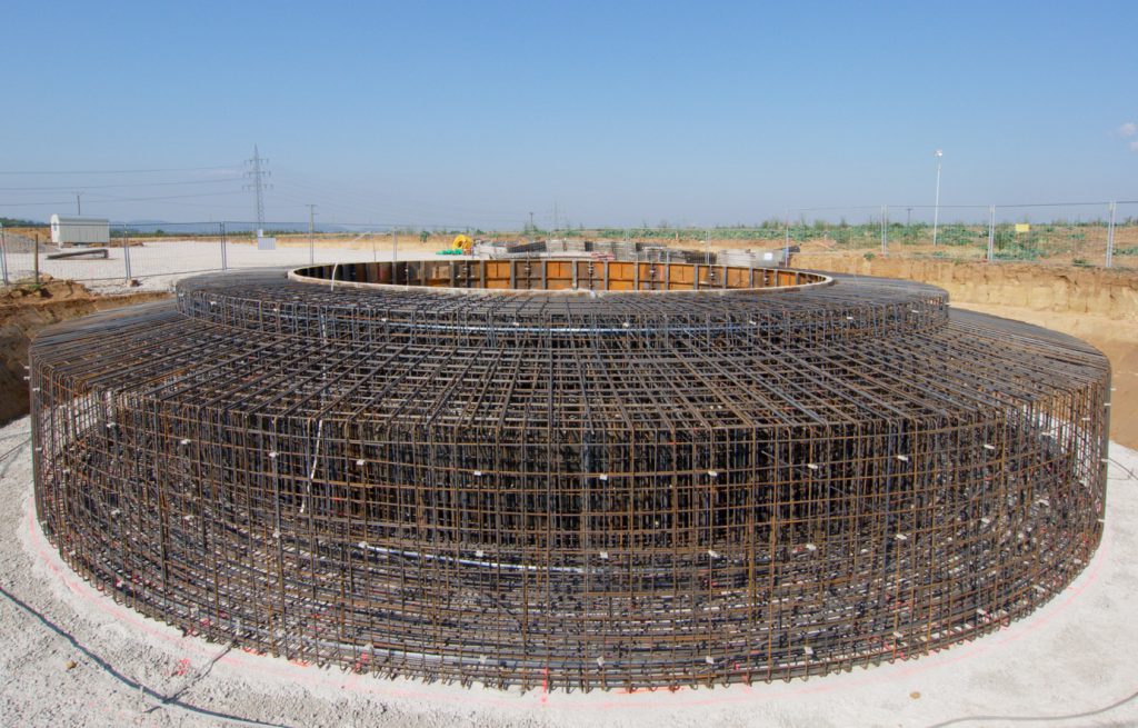
Foundations and access
The areas for the foundations are still the least of the evils, although in Schleswig Holstein alone, a sealed area of 3 million square meters was assumed in 2018. Approximately 1300 cubic meters of concrete and 180 tons of steel disappear in such foundations.
It is not even clear how such colossuses are to be removed from the forest later on, or how they can be removed at all. Anyone who has ever spent a holiday in France on the Atlantic Ocean knows that concrete remains, i.e. bunkers, of the 3rd Reich bunkers stubbornly refuse to decay on the coasts. Ina 1000 years probably only the bunkers of the Nazis or the foundations of wind turbines will remain.
Access to wind turbines is much more serious than the foundations, which only cover a relatively small area. Wind turbines are getting ever taller and the rotors ever bigger. The radius that the special transport vehicles now is so large that a massive quantities of trees have to make way for access roads. And since the wind turbines only have a limited lifetime, the access roads have to remain, because at some point they will have to be dismantled or maintained. The forest at this point is lost and chopped up.
German conservative CDU now poised to play along
The CDU Lower Saxony is now poised to go along with a proposal that more wind turbines in forests should be approved. Whether an impact assessment has been made here? Especially in forests, the population of birds of prey is high and one can only guess what will happen if huge rotors rotate over birds or their breeding grounds and habitat. These rotors are, as studies show, a considerable hazard for birds of prey.
Indeed the wind power lobby is trying to invalidate such studies, for example by pointing out the large number of songbirds and garden birds that are killed annually by windows, cars or cats. But if you use your common sense, here you see whataboutism in its purest form. Birds of prey very rarely die from windows, cars or cats and songbirds and garden birds rarely die from wind turbines. At the latest, when the census of seabirds in the Irish Sea – an area with a lot of wind turbines – shows that the population is declining massively, the windscreen/cat/car argument falls apart.
The same outcome, but completely different reactions
But it gets really crazy when we look at the situation in places like the Reinhardts Forest in the state of Hesse. This forest is very valuable, because it still has a virgin forest character in parts. Nevertheless, wind turbines are to be built there with all the consequences described above. Residents’ protests are being dismissed as an obstacle to technology and energy production transformation.
Yet, at the same time, the people go into collective outrage when the Amazon becomes smaller through slash-and-burn clearing. In both cases forests, biotopes and very same carbon reservoirs are lost, but with completely contrary reactions. Good and bad trees.
Used to be tranquility above the tree tops
But forests are much more. Many people pursue various activities there. A climate activist from Berlin Kreuzberg or Hamburg Ottensen may find this hard to imagine, but there are actually people who visit the forests enjoy tranquility or the sounds of nature. If the plans of wind power advocates are anything to go by, then in many forests this will soon be lost forever.
I see that the merchants of hype are at it again. The scary headline says “Report: Sea-level rise ‘accelerating’ along U.S. coasts, including in the Bay Area“. And in the text, it says “The Bay Area was home to two of those stations: one in Alameda and one in San Francisco, which both recorded a year-over-year rise.” Of course, they blamed the usual suspect, global warming.
I see that and I say … whaaa? I live an hour and a half north of San Franciso, and I’ve been following sea levels around here for a while. I knew nothing of any sea-level acceleration.
The media article references something called the “US Sea Level Report Card“, which indeed lists San Francisco and Alameda. So I went to the NOAA Tides and Currents site to get the data. Let me start with the shorter of the two datasets, Alameda. It’s an island, albeit just barely, in San Francisco Bay near Oakland. It’s lovely, I lived there on the waterfront for a bit just after I got married.
Originally it was part of the Oakland mainland, but in the 1890s the canal at the lower right was cut through. This allowed flowing water to prevent the ongoing problem with siltation in that estuary. As a consequence, the land across from the island became the main location for the Port of Oakland. The channel between Alameda and the mainland is a gorgeous part of the world. Here’s a photo I took the last time I sailed those waters, showing the giant land horses of the Port.
So what is the story of the Alameda sea levels? Here you go:
Figure 1. Sea level in Alameda, California. The red line is an 8-year centered Gaussian average, the blue line is the linear trend
Hmm … not seeing a whole lot of acceleration in that record. It might show as acceleration, however, because it both starts and ends at a high point.
The oddity of this sea-level record is that it’s not far from San Francisco, but the sea level rise is less than half that of SF … say what? Must be some vertical movement of the land itself, go figure. It can’t be an actual real difference in sea level, otherwise compared to 1939, after 80 years the sea level in Alameda would permanently be some four inches (100 mm) lower than the level ten miles (16 km) across the bay. Not possible.
Based on that impossiblity, I’d advise not putting any weight on the Alameda record … but I digress.
How about San Francisco? It has a much longer record, so any acceleration should be more visible. Here’s that graph:
Figure 2. Sea level in San Francisco, California. The red line is an 8-year centered Gaussian average, the blue line is the linear trend
Man, that is about as straight a line as anyone could want.
Mystified by the claims of acceleration, I went to see how the “Sea Level Report Card” study accelerated the acceleration. Turns out the answer is simple.
1) Throw away all of the data before 1969.
2) Calculate a quadratic (accelerating) fit to the data.
3) Subject it to bootstrap and Monte Carlo tests to see if it’s significant.
4) Extend the quadratic fit out to the year 2050
5) Declare success.
Seriously, that’s what they’ve done. Here’s their “Sea Level Report Card” for Alameda, starting in 1969:
Figure 3. Alameda graph from the study. Projection of unverified acceleration out to 2050.
Figure 4. San Francisco graph from the study. Projection of unverified acceleration out to 2050.
As you can see from the graphs, in both cases the quadratic (accelerating) trend is only trivially different in the period covered by the actual data. The two lines overlap almost entirely during that period. Occams Razor says don’t unnecessarily multiply causes. And by that maxim, a straight line is the better choice. But Occam has been wrong more than once …
So to avoid getting a bad shave from Occam, I ran my usual analysis on both datasets. Using the full-length datasets in both cases, I started by looking at the Hurst Exponent of the datasets. The Hurst Exponent varies from 0 to 1, with random datasets measuring 0.5. It measures how “autocorrelated” the data is, meaning how much this month is like last month, this year is like last year, this decade is like last decade.
And the problem is that when the Hurst Exponent is high, it means the data is naturally trendy, so that large swings up and down are not uncommon. See here for a discussion of the issues.
In both cases, the Hurst Exponent is high — 0.77 for Alameda and 0.73 for SFO. This is plenty large enough to invalidate normal statistical tests.
And speaking of tests, the normal statistical test (ANOVA) shows that for San Francisco, the accelerating “Quadratic Trend” seen in Figure 1 is not statistically better than just a straight line.
However, the situation is different for Alameda. The ANOVA test shows that the Quadratic Trend does a significantly better job than a straight line in explaining the data.
Ah, but the Hurst Exponent … let me take a small digression.
The number of months or other data points in a dataset is usually represented by “N”. For San Francisco, there are 1,896 months of data, so N = 1,896. That’s lots of data points, which is good. It makes any conclusions that we draw more solid. It reduces the uncertainty in trends and the like. The more data points we have, the better.
The normal way to deal with a high Hurst Exponent dataset is to calculate an “effective N” which reflects the number of normal random data points that the dataset will act like. I use the method of Koutsoyiannis to calculate effective N, as I described in the link above. And I discussed the question of sea levels and effective N here.
For the San Francisco data, instead of the N of 1,896 months of data (data points), the effective N turns out to be only 57 data points.
And since we couldn’t say that the Quadratic Trend is a better fit with 1,896 data points … there is no chance of it being statistically significant with only 57.
Regarding Alameda, it has an N of 969 months. But when we calculate the effective N, it’s only 24. And while (unlike San Francisco) the ANOVA test showed the Alameda accelerating Quadratic Trend was significantly better without adjusting for autocorrelation, once we take the Hurst Exponent into account, the acceleration is no longer significant.
Of course, when they chop off the early part of both records before 1969, it just gets worse. Both datasets now have only 612 data points … and the effective N is only 12 for Alameda and 14 for San Francisco. And with that small an N, all bets are off—it’s far, far too little data to come to any conclusions of any kind about small levels of acceleration.
Now me, in addition to looking at the statistical calculations, I use another method. Recently I realized that we can employ an unusual application of Complete Ensemble Empirical Mode Decomposition analysis, also known as “CEEMD”, to the sea level question. CEEMD breaks down (“decomposes”) any signal into its component cycles by frequency bands. It removes these bands of cycles (known as “empirical modes”), one at a time, from the signal. At the end of the process, what’s left behind is the part without cycles, called the “residual”. My insight was that we can look at that residual to understand the most basic swings in the tidal dataset after all the natural tidal cycles are removed.
The CEEMD method is classed as a “noise-assisted” method of data analysis, which seems like a contradiction in terms. For those unfamiliar with the method, I wrote about it here.
So let’s see how the CEEMD works out in practice. Here is the Complete Ensemble Empirical Mode Decomposition (CEEMD) of the San Francisco dataset.
Figure 3. CEEMD decomposition of the San Francisco tide levels. The top panel shows the raw annual sea level data. Empirical Modes C1 to C5 show the component cycles starting with the highest frequency (shortest period) cycles and working down to the lowest frequency (longest period). The bottom panel shows the residual that’s left once C1 through C5 are subtracted from the raw data. The individual Empirical Modes actually have different amplitudes, but I’ve set them all to the same size for easy comparison. Units are Standard Deviations.
We can take another look at this same decomposition in a “periodogram” that shows the lengths and strengths of the cycles.
Figure 4. This shows the periods of the various Empirical Modes C1 through C5. As you can see, there are strong cycles at about 13 years (Mode C4), and 27 and 36 years, with smaller cycles centered at 50 and 80 years (Mode C5).
As I said, the relevant graph for our purposes is the “Residual” shown as the bottom panel in Figure 3. This is what’s left after all tidal cycles are removed. As we’ve seen, there are significant cycles in the San Francisco data out to around fifty years and more. This generally agrees with Mitchell’s conclusion in “Sea Level Rise in Australia and the Pacific” who noted (see p. 15) that even after 50 years, sea-level rise accuracy is still only ± a couple of mm. This is because the tides have long, slow oscillations, and if we use shorter data, we may just be looking at a tidal cycle rather than a true sea-level change.
So here’s how I plot up the CEEMD residual. I overlay it on the linear trend of the residual so I can see just how the residual changes over time. Here’s that graph.
Figure 5. The “residual” of the CEEMD analysis of the San Francisco sea level data, what remains after all cycles have been removed from the data.
As you can see, once we remove the tidal cycles from the data there is no acceleration. However, I suspect that the authors of the study have mistaken the slight increase in trend from the relatively level period 1975-2000 for acceleration. Go figure.
How about Alameda? Here’s the CEEMD data:
Figure 6. As in Figure 4, for the Alameda data.
And here are the periodograms of the Alameda Empirical Modes:
Figure 7. This shows the periods of the various Empirical Modes C1 through C5. As you can see, there are strong cycles in the range from 10 to 15 years, and around 30 years.
Here we can see the problem with even a 60-year dataset. There’s still energy in cycle lengths all the way out to 60 years, so we’re unable to truly disentangle the trend from the cycles. However, given that, here’s the residual.
Figure 8. CEEMD residual, as in Figure 5, but for Alameda Island
YIKES! You can see what I meant about problems with the Alameda data. I suspect it has to do with the groundwater levels. I find the following:
From the 1850’s, Alameda Island had been known for its abundant, pure water supply. Early wells varied in depth from a few feet to hundreds of feet deep. Even in the early days, it was common knowledge that artesian waters would be found along the southwestern side of the island at a depth of 100 feet or so. The water would rise in the bore holes to about high tide level. SOURCE
So obviously, there is trapped water a hundred feet under the island exerting significant upward pressure. Since then, these wells have been pumped, and then shut down, and new wells drilled, and pumped, and then shut down. In addition, the island was a Naval Air Base during the war, and the population and the water use varied greatly before and after. My guess is that what we are seeing in the Alameda sea-level record are changes in land level resulting from changes in groundwater pressure.
Intrigued, I thought I’d look further. Here’s the sea-level record for San Diego, California.
To my surprise, a standard analysis shows a very slight acceleration over the period. The rate of sea-level rise is increasing by a hundredth of a millimetre (0.01 mm) per year … be still, my beating heart. Almost too small to measure.
And in fact, we can kinda see this very small acceleration in the CEEMD analysis.
Figure 10. CEEMD residual, as in Figure 5, but for San Diego
This shows why I like my CEEMD method of looking at sea levels. The residual, showing the underlying changes in the rate of sea-level rise, starts out above the trend line. For forty years, from 1920 to 1960, it is a straight line exactly on the trend. It then decreases slightly and slowly for about 20 years, when it starts to increase, once again slightly and slowly. And at the end of the period, it appears to be slowing down again.
Is this a true acceleration of the rate of sea-level rise in San Diego? Well … I’d say no. I’d say that we are seeing very slight increases and decreases in the rate, but that they are not statistically significant. And the analysis using the Hurst Exponent to calculate “effective N” says the same thing—with an effective N of only 19, there is no statistically significant acceleration in the San Diego sea-level record.
CONCLUSIONS:
• There is no significant acceleration of any kind in the San Francisco tide level data.
• Due to changes in ground level, the Alameda tide station is completely unsuited for any kind of comparison to other sites or for projections into the future. However, I can understand why the authors of the “Sea Level Report Card” study might mistakenly think that it is accelerating …
• The San Diego record shows a very slight acceleration, but it is not significant when corrected for autocorrelation. It also appears not to be a true acceleration, but instead a slight “porpoising” above and below the trend line.
• Whatever method the authors are using to determine if there is significant acceleration seems to be giving false positives.
• Despite being warned about upcoming dangerous sea-level acceleration by societies of very learned folks and by climate alarmists since the 1980s, and despite claims that major cities would be underwater by 2020 or 2050, there is still no sign of such threatening sea-level rise. In particular, the ocean around San Francisco has been rising both slowly and steadily with very little variation for over 160 years.
And here in our house up atop the first major ridge in from the coast, on this lovely sunny spring day I gaze out upon a small bit of the distant ocean visible between the hills, whose level keeps rising at its historical pace of about eight inches per century.
My very best wishes to you all,
w.
PS – Just for humor’s sake, here’s their “Sea Level Report Card” from Crescent City, at the northernmost end of the California Coast.
According to their report card, the rate of rise is accelerating … in the wrong direction. Looks like no drowned cities up there …
PPS: As is my wont, I politely request that when you comment, you quote the exact words you are discussing so we can all be clear on your subject.
Anthony has pointed out the further inanities of that well-known vanity press, the Proceedings of the National Academy of Sciences. This time it is Michael Mann (of Hockeystick fame) and company claiming an increase in the rate of sea level rise (complete paper here, by Kemp et al., hereinafter Kemp…
In my previous post I discussed some of the issues with the paper “Climate related sea-level variations over the past two millennia” by Kemp et al. including Michael Mann (Kemp 2011). However, some commenters rightly said that I was not specific enough about what Kemp et al. have done wrong,…
Much has been made in AGW circles of the sea level forecast of Vermeer and Rahmstorf, in “Global sea level linked to global temperature” (V&R2009). Their estimate of forecast sea level rise was much larger than that of the IPCC Fourth Assessment Report (FAR). Their results have been hyped at…
Well, I started a post on Kiribati, but when it was half written I found Andi Cockroft had beaten me to it with his post. His analysis was fine, but I had a different take on the events. President Tong of Kiribati says the good folk of the atolls are…
In a post here on WUWT, Nils-Axel Morner has discussed the sea level in Kwajalein, an atoll in the Marshall Islands. Sea levels in Kwajalein have been rising at an increased rate over the last 20 years. Nils-Axel pointed to a nearby Majuro tidal record extending to 2010, noting that…
Among the recent efforts to explain away the effects of the ongoing “pause” in temperature rise, there’s an interesting paper by Dr. Anny Cazenave et al entitled “The Rate of Sea Level Rise”, hereinafter Cazenave14. Unfortunately it is paywalled, but the Supplementary Information is quite complete and is available here.…
Science Magazine is published by the American Association for the Advancement of Science. I’m reading my AAAS Newsletter, and I find the following blurb (emphasis mine): Virginia Panel Releases Coastal Flooding Report. A subpanel of the Secure Commonwealth Panel of Virginia released a report containing several recommendations for dealing with risks…
[see update] Well, the claims of the ‘first climate refugees’ are coming up again. I think we’re up to the ninth first climate refugees, it’s hard to keep track. In any case, I came across this: International leaders gathering in Paris to address global warming face increasing pressure to tackle …
(NOTE UPDATE AT END) There’s a recent and good post here at WUWT by Larry Kummer about sea level rise. However, I disagree with a couple of his comments, viz: (b) There are some tentative signs that the rate of increase is already accelerating, rather than just fluctuating. But the …
I got to thinking about the records of the sea level height taken at tidal stations all over the planet. The main problem with these tide stations is that they measure the height of the sea surface versus the height of some object attached to the land … but the …
Nerem and Fasullo have a new paper called OBSERVATIONS OF THE RATE AND ACCELERATION OF GLOBAL MEAN SEA LEVEL CHANGE, available here. In it, we find the following statement: …
With apologies to Paul Revere, this post is on the lookout for cooler weather with an eye on both the Land and the Sea. UAH has updated their tlt (temperatures in lower troposphere) dataset for January 2020. Previously I have done posts on their reading of ocean air temps as a prelude to updated records from HADSST3. This month also has a separate graph of land air temps because the comparisons and contrasts are interesting as we contemplate possible cooling in coming months and years.
Presently sea surface temperatures (SST) are the best available indicator of heat content gained or lost from earth’s climate system. Enthalpy is the thermodynamic term for total heat content in a system, and humidity differences in air parcels affect enthalpy. Measuring water temperature directly avoids distorted impressions from air measurements. In addition, ocean covers 71% of the planet surface and thus dominates surface temperature estimates. Eventually we will likely have reliable means of recording water temperatures at depth.
Recently, Dr. Ole Humlum reported from his research that air temperatures lag 2-3 months behind changes in SST. He also observed that changes in CO2 atmospheric concentrations lag behind SST by 11-12 months. This latter point is addressed in a previous post Who to Blame for Rising CO2?
After a technical enhancement to HadSST3 delayed March and April updates, May resumed a pattern of HadSST updates mid month. For comparison we can look at lower troposphere temperatures (TLT) from UAHv6 which are now posted for January. The temperature record is derived from microwave sounding units (MSU) on board satellites like the one pictured above. Recently there was a change in UAH processing of satellite drift corrections, including dropping one platform which can no longer be corrected. The graphs below are taken from the new and current dataset.
The UAH dataset includes temperature results for air above the oceans, and thus should be most comparable to the SSTs. There is the additional feature that ocean air temps avoid Urban Heat Islands (UHI). The graph below shows monthly anomalies for ocean temps since January 2015. After a June rise in ocean air temps, all regions dropped back down to May levels in July and August. A spike occured in September, followed by plummenting October ocean air temps in the Tropics and SH. In November that drop partly warmed back, now leveling slightly downword with continued cooling in NH. 2020 starts with NH warming slightly, still cooler than the previous months back to September. SH and Tropics also rose slightly resulting in a Global rise.
Land Air Temperatures Cooling in Seesaw Pattern
We sometimes overlook that in climate temperature records, while the oceans are measured directly with SSTs, land temps are measured only indirectly. The land temperature records at surface stations sample air temps at 2 meters above ground. UAH gives tlt anomalies for air over land separately from ocean air temps. The graph updated for January 2020 is below.
Here we have freash evidence of the greater volatility of the Land temperatures, along with an extraordinary departure by SH land. Despite the small amount of SH land, it spiked in July, then dropped in August so sharply along with the Tropics that it pulled the global average downward against slight warming in NH. In November SH jumped up beyond any month in this period. Despite this spike along with a rise in the Tropics, NH land temps dropped sharply. The larger NH land area pulled the Global average downward. December reversed the situation with the SH dropping as sharply as it rose, while NH rose to the same anomaly, pulling the Global up slightly.
2020 starts with sharp drops in both SH and NH, with the Global anomaly dropping as a result. The behavior of SH land temps is puzzling, to say the least. it is also a reminder that global averages can conceal important underlying volatility.
The longer term picture from UAH is a return to the mean for the period starting with 1995. 2019 average rose but currently lacks any El Nino to sustain it.
TLTs include mixing above the oceans and probably some influence from nearby more volatile land temps. Clearly NH and Global land temps have been dropping in a seesaw pattern, more than 1C lower than the 2016 peak, prior to these last several months. TLT measures started the recent cooling later than SSTs from HadSST3, but are now showing the same pattern. It seems obvious that despite the three El Ninos, their warming has not persisted, and without them it would probably have cooled since 1995. Of course, the future has not yet been written.