Month: May 2023

Fake meat could make 25 times more CO2 than real beef

By Jo Nova

It turns out that replicating a cow in a laboratory is not as simple as expected. A new study points at some very major and potentially very hard to solve problems with lab meat. We can scale up bacteria in factories easily, but animal cells are very different. Muscle cells not only need a sterile complicated broth but they are basically a sitting-duck feast for any bacteria.

Quote of the day:

“USD 2 billion has already been invested in this technology, but we don’t really know if it will be better for the environment,” Risner said.

Think of a cow as being an entire industrial production campus for meat — to deal with chemical toxins it comes with a customized chemical factory (a liver) and two industrial filter systems (kidneys), and a full immune defense force on a 24 hour watch to deal with the constant flood of microbial contaminants. Cows also have nutrient intake systems to break down grass into separate  chemical components which are stored, transported and chemically tweaked to suit. All departments are self repairing, and are equipped with their own laboratory testing, messaging and alert service. The sterile growth conditions of muscle are maintained most of the time in close proximity to dirt and poo. The biological machinery has been road-tested and refined for a half a billion years. Yet somehow we thought we could replicate all that and do it more efficiently in a couple of decades.

Instead of thirty factories, 200 labs, 2000 trucks and sterilized vats of heated pharmaceutical grade goo, we could just use a cow.

It takes a lot of energy to replicate a cow

It’s not enough to kill bacteria in the growth broth, we have to remove the dead body parts of the bacteria too. The outside shell of many bacteria breaks up into is what we call an endotoxin. You may not know it but these are just bad, bad, bad — they are lipopolysaccarides that sometimes leak from our intestinal walls and trigger fever, nausea, inflammation, shivering and shock. So the dead parts of bacteria have to be cleaned out of the broth — which means chromatography, or ultrafiltration, or ion exchanges, and fine membranes. All of which uses lots of energy.

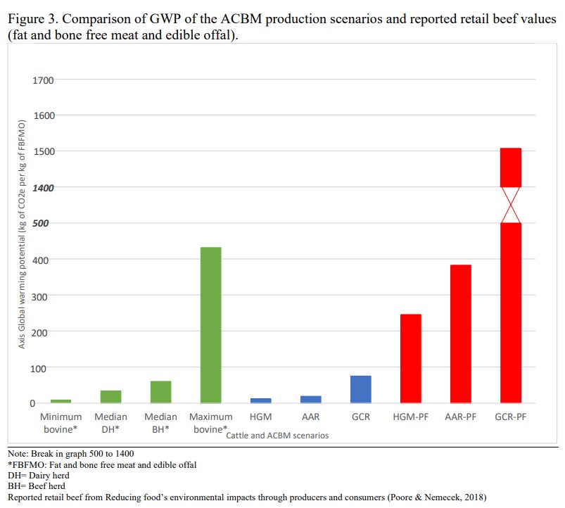
Fake meat practically eats fossil fuels:

The three red bars on the right are different scenarios for creating growth mediums. The PF stands for Purification Factor (meaning highly purified).

Environmental impacts of cultured meat: A cradle-to-gate life cycle assessment

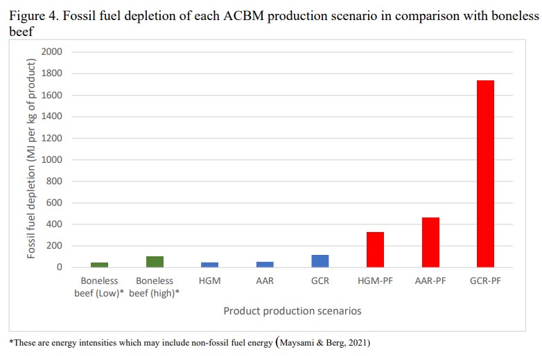
GWP means Global Warming Potential. ACBM means fake meat or “Animal Cell-Based Meat”.BH means Beef Herd, and DH means Dairy.  Risner et al

Would you like global warming with your burger?

Note the scale on the vertical axis.

TVP World

The broth itself must contain salts, sugars, amino acids, and vitamins, and the production of each of these elements involves an expenditure of energy.

This “pharmaceutical” level of purification is essential as animal cells will not grow in a broth that is “contaminated” with bacteria. Experts involved in improving the process are testing to what extent it is possible to move away from purification.

The paper’s first author, Derrick Risner of the University of California (U.S.), in a commentary for “New Scientist”, expressed doubt that moving away from “pharmaceutical” levels of broth purification would be possible since even trace levels of contamination can destroy animal cell cultures.

From the paper — we used to use serum from baby cow blood to grow cells in culture but that is an 18 step process and energy intensive…

Animal cell culture is inherently different than culturing bacteria or yeast cells due to their enhanced sensitivity to environmental factors, chemical and microbial contamination. This can be illustrated by the industrial shift to single use bioreactors for monoclonal antibody production to reduce costs associated with contamination (Jacquemart et al., 2016). Animal cell growth mediums have historically utilized fetal bovine serum (FBS) which contains a variety of hormones and growth factors (Jochems et al., 2002). Serum is blood with the cells, platelets and clotting factors removed. Processing of FBS to be utilized for animal cell culture is an 18-step process that is resource intensive due to the level of refinement required for animal cell culture. Thus, the authors believe that commercial production of an ACBM product utilizing  FBS or any other animal product to be highly unlikely given this high level of  refinement.

The authors say they might be underestimating the costs.

The requirement of endotoxin removal would also contribute to the environmental impact of ACBM products which makes our LCIA results for the minimum scenarios to be underestimated minimums. Utilization of commodity grade growth medium components such as glucose for animal cell growth is unlikely unless the components undergo an endotoxin separation process. The effect of endotoxin can vary greatly depending on cell type and source; however 25 ng/ml of endotoxin was shown to cause cell apoptosis when coupled with non-lethal heat shock (Corning, 2020).

Endotoxins kill cells at just 25 nanograms per ml. The purity required in a complicated mixture on a commerical scale needs Olympic level chemistry. It’s like feeding pharmaceutical grade drugs to your cows instead of grass. This isn’t going to scale up well.

REFERENCE

Risner et al (2023) Environmental impacts of cultured meat: A cradle-to-gate life cycle assessment, bioRXIV, bioRxiv preprint doi: https://ift.tt/67UGFLM;

h/t Another Ian, John Connor II and Climate Depot


10 out of 10 based on 1 rating

via JoNova

https://ift.tt/bn4hEgi

May 12, 2023 at 03:30PM

UAH Air Temps Warming Little in April 2023

The post below updates the UAH record of air temperatures over land and ocean. Each month and year exposes again the growing disconnect between the real world and the Zero Carbon zealots.  It is as though the anti-hydrocarbon band wagon hopes to drown out the data contradicting their justification for the Great Energy Transition.  

As an overview consider how recent rapid cooling  completely overcame the warming from the last 3 El Ninos (1998, 2010 and 2016).  The UAH record shows that the effects of the last one were gone as of April 2021, again in November 2021, and in February and June 2022  Now at year end 2022 and continuing into 2023 global temp anomaly is matching or lower than average since 1995, an ENSO neutral year. (UAH baseline is now 1991-2020).

For reference I added an overlay of CO2 annual concentrations as measured at Mauna Loa.  While temperatures fluctuated up and down ending flat, CO2 went up steadily by ~60 ppm, a 15% increase.

Furthermore, going back to previous warmings prior to the satellite record shows that the entire rise of 0.8C since 1947 is due to oceanic, not human activity.

gmt-warming-events

The animation is an update of a previous analysis from Dr. Murry Salby.  These graphs use Hadcrut4 and include the 2016 El Nino warming event.  The exhibit shows since 1947 GMT warmed by 0.8 C, from 13.9 to 14.7, as estimated by Hadcrut4.  This resulted from three natural warming events involving ocean cycles. The most recent rise 2013-16 lifted temperatures by 0.2C.  Previously the 1997-98 El Nino produced a plateau increase of 0.4C.  Before that, a rise from 1977-81 added 0.2C to start the warming since 1947.

Importantly, the theory of human-caused global warming asserts that increasing CO2 in the atmosphere changes the baseline and causes systemic warming in our climate.  On the contrary, all of the warming since 1947 was episodic, coming from three brief events associated with oceanic cycles. 

Update August 3, 2021

Chris Schoeneveld has produced a similar graph to the animation above, with a temperature series combining HadCRUT4 and UAH6. H/T WUWT

image-8


mc_wh_gas_web20210423124932

See Also Worst Threat: Greenhouse Gas or Quiet Sun?

April 2023 Update  Land and Sea Temps Little Changed

banner-blog

With apologies to Paul Revere, this post is on the lookout for cooler weather with an eye on both the Land and the Sea.  While you will hear a lot about 2020-21 temperatures matching 2016 as the highest ever, that spin ignores how fast the cooling set in.  The UAH data analyzed below shows that warming from the last El Nino was fully dissipated with chilly temperatures in all regions. After a warming blip in 2022, land and ocean temps dropped again with 2023 starting below the mean since 1995.

UAH has updated their tlt (temperatures in lower troposphere) dataset for April 2023. Posts on their reading of ocean air temps this month came ahead of updated records from HadSST4.  I just posted on SSTs using HadSST4 El Nino Comes to Save Global Warming April 2023 This month also has a separate graph of land air temps because the comparisons and contrasts are interesting as we contemplate possible cooling in coming months and years. Sometimes air temps over land diverge from ocean air changes.  For example in February, Tropical ocean temps alone moved upward, while temps in all land regions rebounded after hitting bottom..

Note:  UAH has shifted their baseline from 1981-2010 to 1991-2020 beginning with January 2021.  In the charts below, the trends and fluctuations remain the same but the anomaly values change with the baseline reference shift.

Presently sea surface temperatures (SST) are the best available indicator of heat content gained or lost from earth’s climate system.  Enthalpy is the thermodynamic term for total heat content in a system, and humidity differences in air parcels affect enthalpy.  Measuring water temperature directly avoids distorted impressions from air measurements.  In addition, ocean covers 71% of the planet surface and thus dominates surface temperature estimates.  Eventually we will likely have reliable means of recording water temperatures at depth.

Recently, Dr. Ole Humlum reported from his research that air temperatures lag 2-3 months behind changes in SST.  Thus the cooling oceans now portend cooling land air temperatures to follow.  He also observed that changes in CO2 atmospheric concentrations lag behind SST by 11-12 months.  This latter point is addressed in a previous post Who to Blame for Rising CO2?

After a change in priorities, updates are now exclusive to HadSST4.  For comparison we can also look at lower troposphere temperatures (TLT) from UAHv6 which are now posted for March.  The temperature record is derived from microwave sounding units (MSU) on board satellites like the one pictured above. Recently there was a change in UAH processing of satellite drift corrections, including dropping one platform which can no longer be corrected. The graphs below are taken from the revised and current dataset.

The UAH dataset includes temperature results for air above the oceans, and thus should be most comparable to the SSTs. There is the additional feature that ocean air temps avoid Urban Heat Islands (UHI).  The graph below shows monthly anomalies for ocean air temps since January 2015.


Note 2020 was warmed mainly by a spike in February in all regions, and secondarily by an October spike in NH alone. In 2021, SH and the Tropics both pulled the Global anomaly down to a new low in April. Then SH and Tropics upward spikes, along with NH warming brought Global temps to a peak in October.  That warmth was gone as November 2021 ocean temps plummeted everywhere. After an upward bump 01/2022 temps reversed and plunged downward in June.  After an upward spike in July, ocean air everywhere cooled in August and also in September.   After sharp cooling everywhere in January 2023, all regions were into negative territory. Now in February, March and April, an uptick in the Tropics led to a small rise globally slightly above zero. Unusually SH, NH and Global anomalies are all the same 0.17.

Land Air Temperatures Tracking Downward in Seesaw Pattern

We sometimes overlook that in climate temperature records, while the oceans are measured directly with SSTs, land temps are measured only indirectly.  The land temperature records at surface stations sample air temps at 2 meters above ground.  UAH gives tlt anomalies for air over land separately from ocean air temps.  The graph updated for April is below.

Here we have fresh evidence of the greater volatility of the Land temperatures, along with extraordinary departures by SH land.  Land temps are dominated by NH with a 2021 spike in January,  then dropping before rising in the summer to peak in October 2021. As with the ocean air temps, all that was erased in November with a sharp cooling everywhere.  After a summer 2022 NH spike, land temps dropped everywhere, and in January, further cooling in SH and Tropics offset by an uptick in NH.  Now in February and March both SH and Tropics along with NH pulled up the Global land anomaly.

The Bigger Picture UAH Global Since 1980

The chart shows monthly Global anomalies starting 01/1980 to present.  The average monthly anomaly is -0.06, for this period of more than four decades.  The graph shows the 1998 El Nino after which the mean resumed, and again after the smaller 2010 event. The 2016 El Nino matched 1998 peak and in addition NH after effects lasted longer, followed by the NH warming 2019-20.   An upward bump in 2021 was reversed with temps having returned close to the mean as of 2/2022.  March and April brought warmer Global temps, later reversed, and with the sharp drops in Nov., Dec. and January 2023 temps, there was no increase over 1980. Now in February and March there is a slight rebound over zero.

TLTs include mixing above the oceans and probably some influence from nearby more volatile land temps.  Clearly NH and Global land temps have been dropping in a seesaw pattern, nearly 1C lower than the 2016 peak.  Since the ocean has 1000 times the heat capacity as the atmosphere, that cooling is a significant driving force.  TLT measures started the recent cooling later than SSTs from HadSST3, but are now showing the same pattern.  It seems obvious that despite the three El Ninos, their warming has not persisted, and without them it would probably have cooled since 1995.  Of course, the future has not yet been written.


via Science Matters

https://ift.tt/l8tuGWd

May 12, 2023 at 02:36PM

Roald Amundsen tried and failed to tame a polar bear cub in 1920

A short account of polar explorer Roald Amundsen’s failed attempt to tame a polar bear cub he had bought in May 1920 from a trader in the Russian Far East appears today in the Barents Observer. The cub was likely captured after its mother was killed, which was a common practice at a time when polar bears were being slaughtered wholesale throughout the Arctic (Crockford 2019; Honderich 1991; Stirling 2011).

It only took a month for Amundsen to give up his experiment. Below are some excerpts; read the full account here. More photos are here.

One day, during Roald Amundsen’s voyage through the Northeast Passage, Georg Kibisow from the Russian Trading Company came aboard Amundsen’s ship, the Maud. He brought along a polar bear cub that he had caught near Kolyma. He offered the cub to Amundsen, who bought it.

Roald Amundsen named the polar bear cub Marie. He gave her a lot of attention in the hope of taming her so she could pull a sledge. Marie features a lot in Amundsen’s expedition diary and he followed her development closely. Here is a sample of what Amundsen wrote:

It’s not easy to make friends with Marie, but it might work. I carry her now, whenever I want, but I have to make sure I hold onto her head so she can’t bite me. She is constantly fighting with the dogs. This little critter has no fear.

[and later]

I chloroformed Marie to death this morning. I had to abandon any hopes of training her. After grooming and feeding her for a month, this morning, when I brought her milk, she came at me in a ferocious rage. In the hands of an experienced trainer she might have become a bit friendlier, but I had to give up.

Context

Below is a map of the Kolyma district in the Russian Far East, which is essentially the drainage of the Kolyma River. The Kolyma River ends in a broad delta that empties into the East Siberian Sea, near the boundary with the Chukchi Sea. Winters in this region are extremely cold and is where most Arctic sea ice forms (Crockford 2022).

A fuller account of his Northeast Passage voyage is here, with more photos, including this one of Marie the polar bear cub in May 1920, and with one of the dog teams in October 1919:

References

Crockford, S.J. 2019. The Polar Bear Catastrophe That Never Happened. Global Warming Policy Foundation, London.

Crockford, S.J. 2022. Polar bear fossil and archaeological records from the Pleistocene and Holocene in relation to sea ice extent and open water polynyas. Open Quaternary 8(7):1–26.  https://doi.org.10.5334/oq.107

Honderich, J.E. 1991. Wildlife as a hazardous resource: an analysis of the historical interaction of humans and polar bears in the Canadian arctic. MA thesis, University of Waterloo, Ontario.

Stirling, I. 2011. Polar Bears: The Natural History of a Threatened Species. Fitzhenry & Whiteside, Markham, Ontario.

via polarbearscience

https://ift.tt/ZsjLgO8

May 12, 2023 at 02:30PM

Objection! Warming Alarm is Hearsay, Lacking Evidence.

C3 Headlines reports: The Real Climate Science Crisis: The Catastrophic Anthropogenic Global Warming (CAGW) Hypothesis Is Without Scientific Evidence.  Excerpts in italics with my bolds and added images.

For a hypothesis to reach the status of being a legit theory, it requires withstanding the onslaught of observed empirical evidence. The CAGW hypothesis is no such animal.

Known by its more contemporary aliases, such as ”climate crisis,” “climate emergency,” “climate collapse,” or “existential threat,” the CAGW has zero empirical evidence to support it.

Unlike the related hypothesis regarding greenhouse gases (GHG) and global warming, at least the GHG hypothesis has warming global temperature data that somewhat coincides with increasing atmospheric CO2 levels, putting aside the growing possibility that the purported cause-and-effect direction is probably the reverse. [Note:  See Temps Cause CO2 Changes, Not the Reverse. 2023 Update]

In order to reach a CAGW climate disaster, global warming temperatures must change rapidly in an accelerating manner that will initiate a ‘tipping point’ for the climate.

The rapid acceleration would present its occurrence in a continuous increasing of the slope, i.e., trend, of temperatures, such as monthly temperatures. Each subsequent month would represent a greater temperature magnitude increase than the month before, hypothetically.

But those tipping point precursors are not occurring in the real-world climate.

For example, it is agreed by all climate scientists that oceans play a very major role in the world’s climate and its global temperatures due to their being both the world’s largest carbon sink and its largest heat content storage.

However, despite these characteristics, in totality, the global oceans HAVE NOT warmed since the year 2014. And certainly, there is no empirical evidence that oceans exhibit constant temperature increases of magnitude.

Quite the contrary, combined oceans exhibit a regular pattern of temperature decreases and increases, as the adjacent plot of NOAA’s monthly ocean data indicates.

Specifically, this is a plot (dark blue) of moving 5-year temperature changes ending each month of the 60-year period from March 1963 through March 2023.

[Explanation: the first data point is the temperature change for the 60 months ending on March 30, 1963; and the chart’s last temperature change data point is for the five 5 years (i.e. 60 months) ending on March 2023.]

The chart also includes a plot (green) of the moving 60-month CO2 level changes over the same sixty year period, plus a linear trend for both CO2 changes and ocean temperature changes.

The trend of the 60-month CO2 changes significantly exceeds the
slight positive trend of ocean temperature changes by a factor of 117x.

This huge differential undercuts the belief that global warming is primarily the result of GHGs. Which is confirmed by the paltry R^2 of +0.06 – an almost non-existent relationship between 5-year atmospheric CO2 changes and 5-year changes in ocean temperature.

Not only are the large increases in CO2 levels not causing a concerning uptick of temperature change magnitude, it also has not lead to any type of acceleration, per the linear trend since 1963.

Specifically, with a trend of a tiny +0.0001°C, that would project out 20 years to be an increase of 5-year temperature changes to an insignificant amount of +0.024 – definitely not an existential threat of ‘runaway warming’ or a CAGW ‘climate crisis’ as portrayed by bureaucrats, politicians and Hollywood celebrities.

So, if 5 years of increasing amounts of CO2 in the atmosphere barely influence 5-year changes in temperature over a 60-year span, either in magnitude or acceleration rate, then it is highly unlikely that this trace gas would cause a catastrophic climate disaster or an extinction event.

Thus, it is fair to state that for all those scientists pushing a narrative of an imminent climate change catastrophe from CO2 without the requisite empirical evidence, this has become the real climate science crisis facing society.

Notes: Temperature and CO2 data sources.Excel used to calculate 60-mth (5-yr) temperature and CO2 changes; used to calculate the respective trends; used to calculate correlation and r-squared; used to plot the chart.

via Science Matters

https://ift.tt/Y3Pg75s

May 12, 2023 at 01:04PM