Volcanic Rumblings

Guest Post by Willis Eschenbach

I noticed that WUWT has a recent post about an interesting study that has identified the mystery huge volcanic eruption in 1831. Turns out that it comes from a volcano named Zavaritskii on an island in the Northwest Pacific between Japan and Russia.

It’s an impressive scientific achievement, and the authors deserve recognition for solving such a long-standing puzzle.

However, I busted out laughing when I read the underlying study in PNAS, entitled The 1831 CE mystery eruption identified as Zavaritskii caldera, Simushir Island (Kurils).

What made me laugh was their claim that the volcano caused a global temperature drop of 1°C (1.8°F, aka “Nearly Two”). I’ve looked at lots of volcanic eruptions. There are links to my research on eruptions and temperature here. I have found that there is no consistent response in the global average surface temperature. I thought “This should be interesting”. I looked at the study to see what evidence they have.

They use the Berkeley Earth land-only temperature data to verify their claim … the problem is that even using their methods, the Berkeley data doesn’t support their claim. The image and the caption in Figure 1 below are from their study.

Figure 1. ORIGINAL CAPTION: Figure S1: Time series of instrumental temperature anomalies spanning 1790–1840 CE. The period 1831–1833 CE is shaded grey. Instrumental temperature records are from Berkeley Earth [www.berkeleyearth.org, (8)] and show estimated global land average temperatures. These represent annual temperature anomalies relative to the 1790–1807 CE mean (a period without major volcanic eruptions).

Squint as I might at Figure 1, I’m not seeing the 1°C temperature drop post-1831. Not even close.

Plus, the Berkeley data is monthly, but they’re using annual averages. This is throwing away a bunch of valuable data.

So I decided to take a proper look at the temperature record of all the major volcanic eruptions for the last two centuries. This eruption information is kept by the Smithsonian Institute in their Volcanoes of the World database. I used only the largest volcanoes, those with a Volcanic Explosivity Index of 6 or more. Here’s that record, compared to the same Berkeley Earth temperature dataset used in their study.

Figure 2. Large volcanic eruptions and the Berkeley Earth global monthly land surface temperature anomaly record.

Here’s the curious part. Of these 7 large volcanoes, there’s only one that is followed by a clear drop in temperature. That one is Pinatubo, the poster child for the claim that eruptions affect global average surface temperatures. All the rest of these big volcanoes show nothing anomalous. Even the two biggest eruptions, Tambora 1812 and Krakatau 1883, were not followed by global cooling in the Berkeley Earth record. Temperatures actually rose after each of those eruptions.

Anyhow … that’s why I laughed when they said they’d found a 1°C (1.8°F) cooling resulting from the 1831 volcano. I didn’t even have to look at the record above to know the chances were small that a large effect would be visible.

And in the event, Figure 2 shows the Zavaritskii volcano occurred halfway through a cooling period, and the cooling post-volcano and pre-volcano are indistinguishable.

I say that this lack of temperature response to eruptions is explained by my hypothesis that a variety of emergent phenomena work to thermoregulate the earth’s temperature. In particular, when temperatures fall due to say eruptions injecting aerosols into the stratosphere, the climate responds inter alia by cumulus cloud fields and thunderstorms forming later in the day. This allows more sunshine to be absorbed by the surface, which opposes the volcanic cooling.

For a different look at this question of temperature changes due to eruptions, I took a look at the UAH MSU satellite-based atmospheric records. Figure 3 shows eruptions and the temperatures at four different atmospheric levels from the top down—stratosphere, tropopause, middle troposphere, and lower troposphere.

Figure 3. UAH MSU satellite-based atmospheric temperature anomalies, in order of altitude from highest (top panel) down to lowest (bottom panel). Red lines show the dates of eruptions with a Volcanic Explosivity Index (VEI) of 5 or more. Numbers following the names show the VEI of the eruption.

Now, this shows the curious nature of the atmosphere—there is very little correlation between stratospheric temperature anomalies (top panel) and the rest of the lower atmosphere (lower three panels). There are clear indications of the 1982 and 1991 volcanoes in the stratosphere … but by the time that works its way down to the lower troposphere, the situation is quite different. There, only the Pinatubo/Cerro Hudson pair shows a temperature drop following the eruption, and even that is not visibly different from a number of other temperature drops during the period.

And by the time the effect of the eruption-injected stratospheric aerosols makes it down to the surface, we get Figure 4.

Figure 4. A closeup of the recent end of the data shown in Figure 2, with additional eruptions. Vertical red lines show VEI 5 and VEI 6 volcanic eruptions during the satellite era along with the Berkeley Earth global monthly land surface temperature record.

If the Mount St. Helens eruption caused the subsequent cooling, did the El Chichon eruption cause the subsequent warming? Once again we see the ~0.5°C temperature drop after Pinatubo, but other than that, there’s no clear indication that eruptions affect the global average surface temperature.

Yes, I know that this goes against the revealed wisdom. That wisdom says:

Eruption –> Stratospheric SO2 Aerosols –> Increased Albedo –> Less Sunlight –> More Cooling

Sounds logical, but it ignores the fact that the climate is a dynamic system that is constantly changing and adapting to a variety of forcings and factors. The revealed wisdom stops too soon. I say it goes like this:

Eruption –> Stratospheric SO2 Aerosols –> Increased Albedo –> Less Sunlight –> Cooling –> Delayed Formation Of Daily Tropical Cumulus Cloud Fields –> Decreased Albedo –> More Sunlight –> Less Cooling

plus

Eruption –> Stratospheric SO2 Aerosols –> Increased Albedo –> Less Sunlight –> Cooling –> Delayed- or Non-Emergence Of Daily Tropical Thunderstorm Formation –> Decreased Thunderstorm Cooling –> Less Cooling

Both of these emergent phenomena, the daily appearance of sunlight-reflecting tropical cumulus cloud fields and cooling thunderstorms, work to oppose the cooling action of the volcanic stratospheric aerosols, and to prevent large swings in the global surface temperature.

I provide interesting evidence for this hypothesis in my post below.

Sunshine here today, thin, but sunshine nonetheless. I’m going for a walk.

My warmest regards to everyone,

w.

AS ALWAYS, I ask that you quote the exact words you are discussing. This keeps misunderstandings to a minimum.

FURTHER READING: In the post below, I use the “stacking” method to compare the temperature response after volcanic eruptions.


Discover more from Watts Up With That?

Subscribe to get the latest posts sent to your email.

via Watts Up With That?

https://ift.tt/phR2udT

January 7, 2025 at 12:01PM

12/2024 Update–As Temperature Changes, CO2 Follows

Previously I have demonstrated that changes in atmospheric CO2 levels follow changes in Global Mean Temperatures (GMT) as shown by satellite measurements from University of Alabama at Huntsville (UAH). That background post is reprinted later below.

My curiosity was piqued by the remarkable GMT spike starting in January 2023 and rising to a peak in April 2024, and then declining afterward.  I also became aware that UAH has recalibrated their dataset due to a satellite drift that can no longer be corrected. The values since 2020 have shifted slightly in version 6.1, as shown in my recent report  Ocean Leads Cooling UAH December 2024.

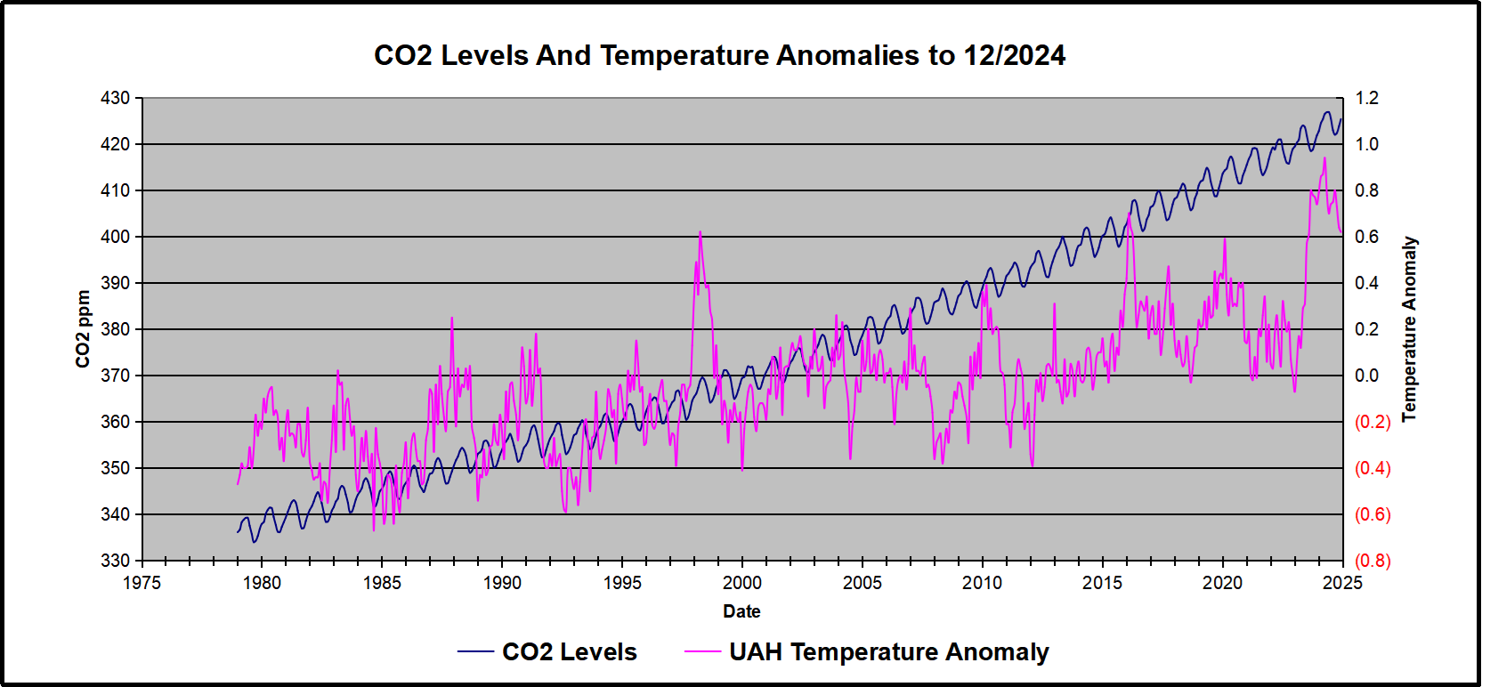
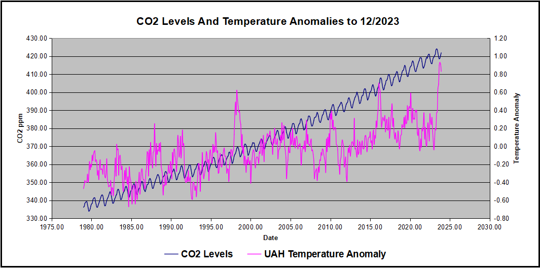
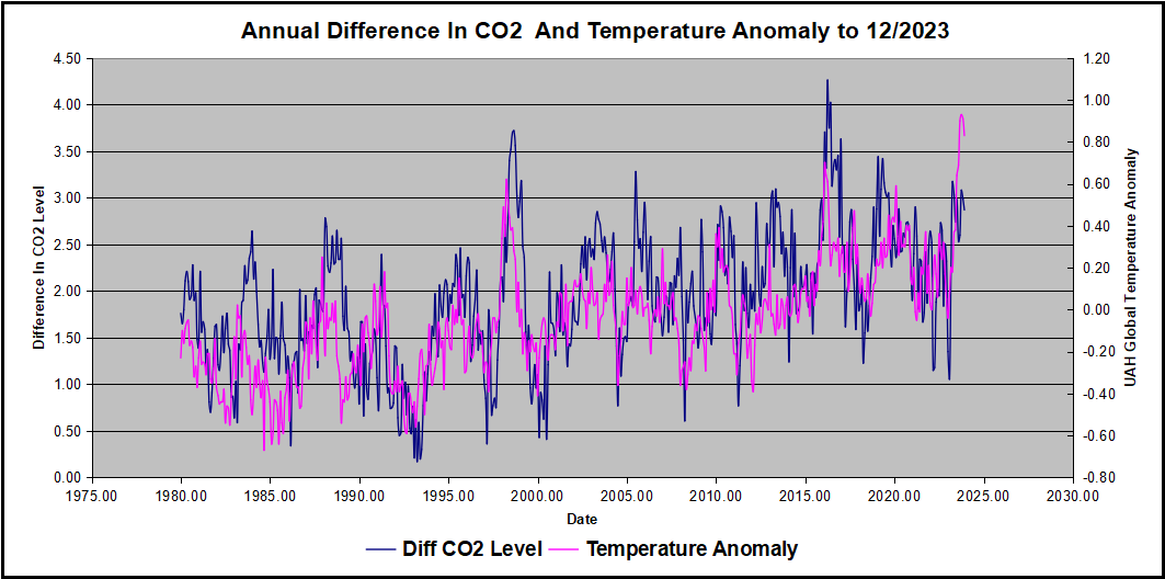
In this post, I test the premise that temperature changes are predictive of changes in atmospheric CO2 concentrations.  The chart above shows the two monthly datasets: CO2 levels in blue reported at Mauna Loa, and Global temperature anomalies in purple reported by UAHv6.1, both through December 2024. Would such a sharp increase in temperature be reflected in rising CO2 levels, according to the successful mathematical forecasting model? Would CO2 levels decline as temperatures dropped following the peak?

The answer is yes: that temperature spike resulted
in a corresponding CO2 spike as expected.
And lower CO2 levels followed the temperature decline.

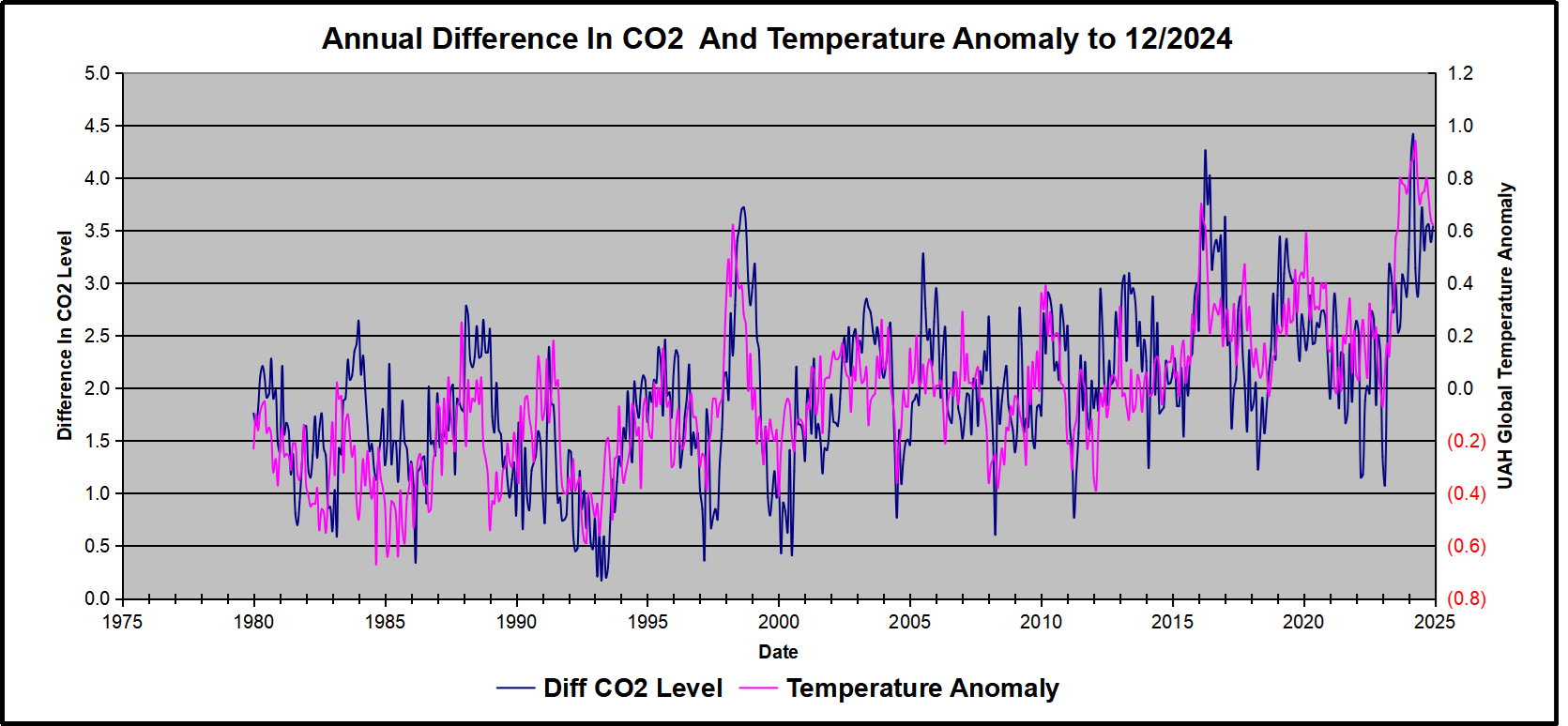
Above are UAH temperature anomalies compared to CO2 monthly changes year over year.

Changes in monthly CO2 synchronize with temperature fluctuations, which for UAH are anomalies now referenced to the 1991-2020 period. CO2 differentials are calculated for the present month by subtracting the value for the same month in the previous year (for example December 2024 minus December 2023).  Temp anomalies are calculated by comparing the present month with the baseline month. Note the recent CO2 upward spike and drop following the temperature spike and drop.

The final proof that CO2 follows temperature due to stimulation of natural CO2 reservoirs is demonstrated by the ability to calculate CO2 levels since 1979 with a simple mathematical formula:

For each subsequent year, the CO2 level for each month was generated

CO2  this month this year = a + b × Temp this month this year  + CO2 this month last year

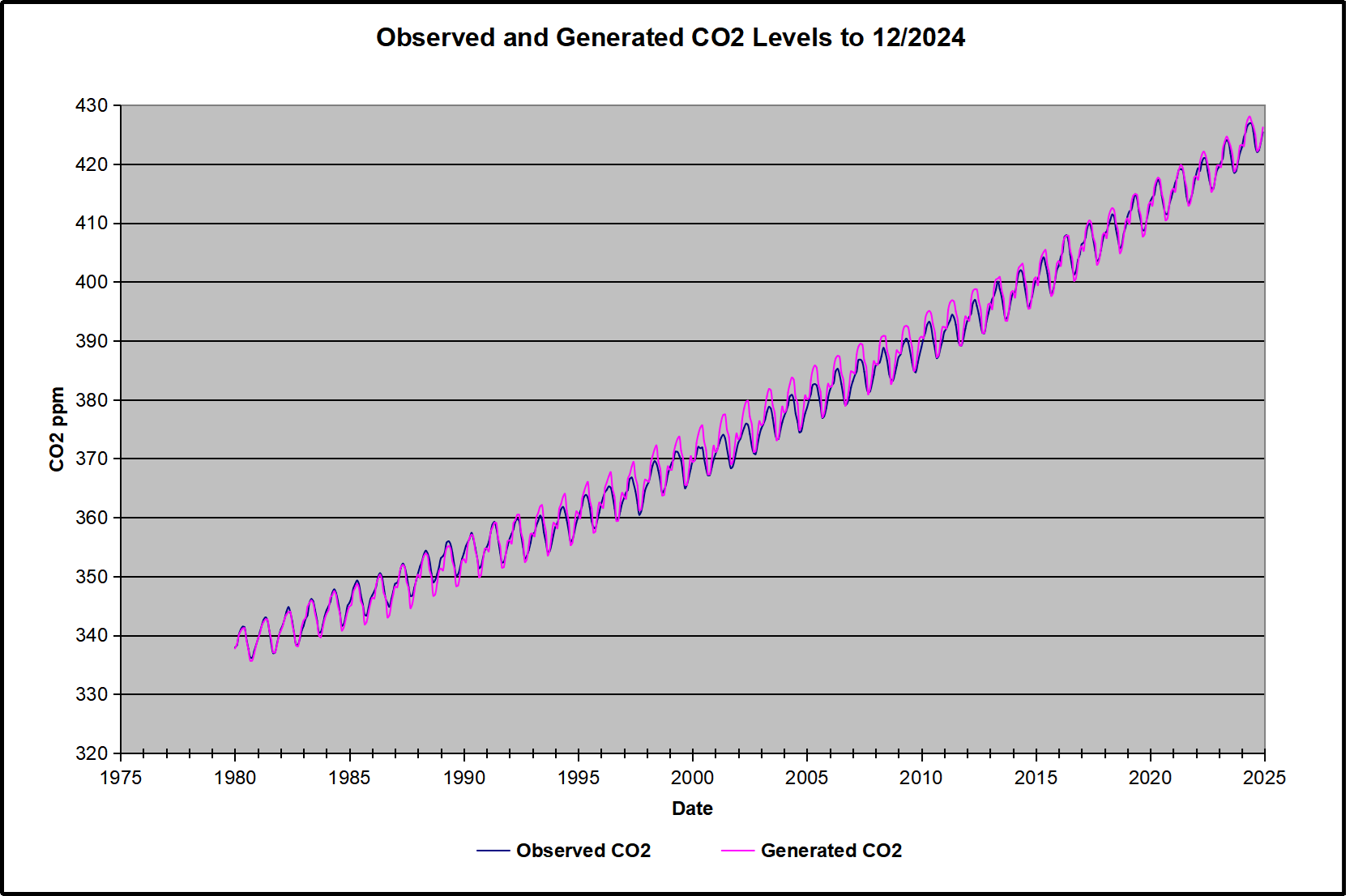
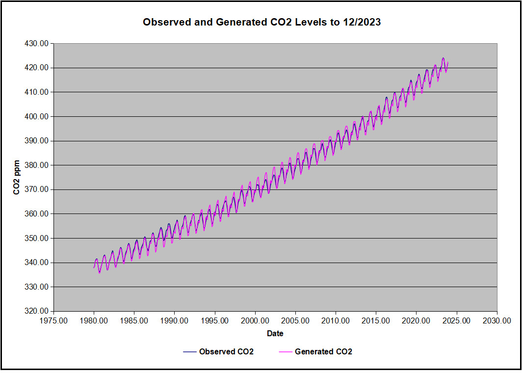
The values for a and b are constants applied to all monthly temps, and are chosen to scale the forecasted CO2 level for comparison with the observed value. Here is the result of those calculations.

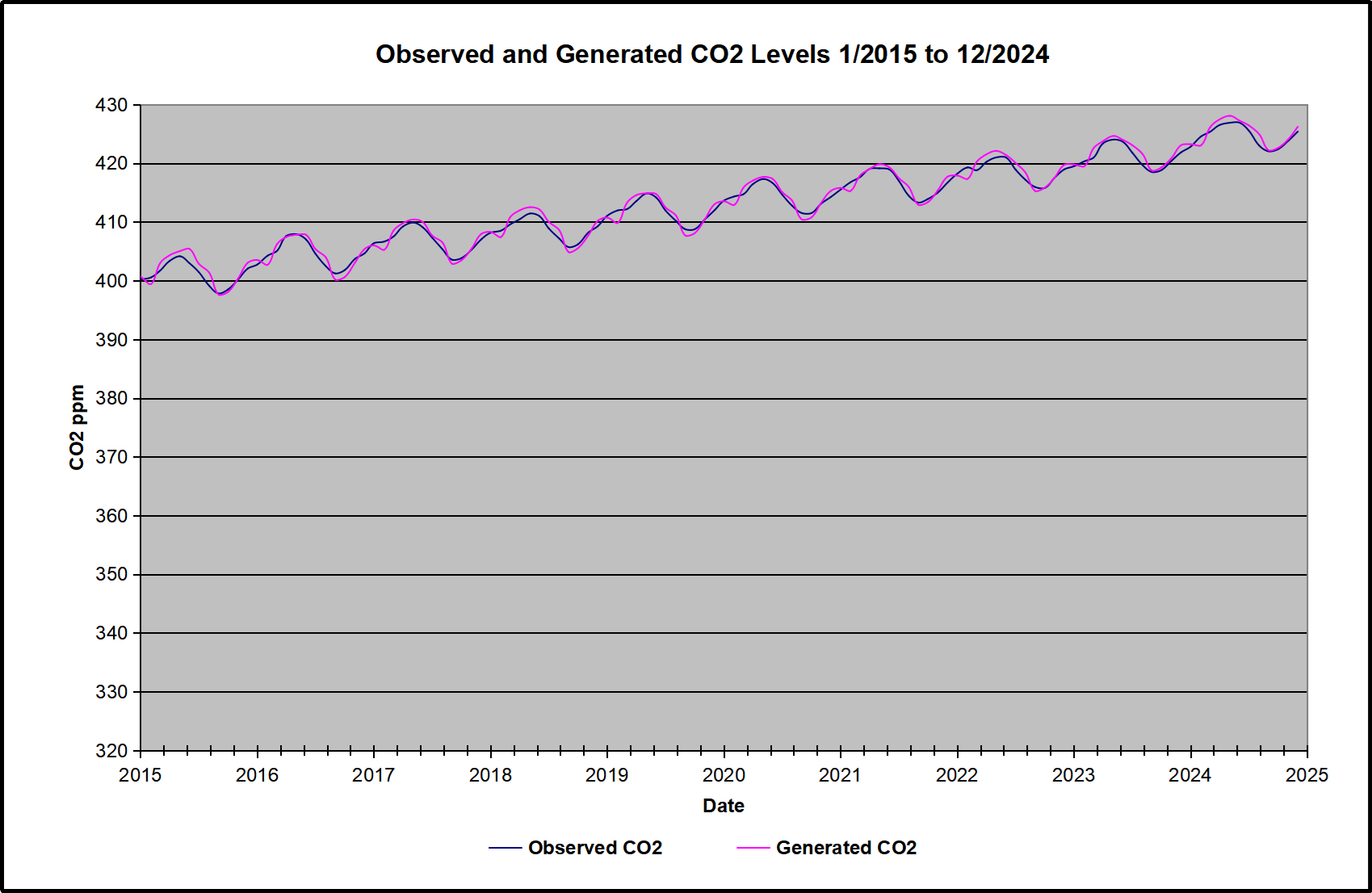
In the chart calculated CO2 levels correlate with observed CO2 levels at 0.9987 out of 1.0000.  This mathematical generation of CO2 atmospheric levels is only possible if they are driven by temperature-dependent natural sources, and not by human emissions which are small in comparison, rise steadily and monotonically.  For a more detailed look at the recent fluxes, here are the results since 2015, an ENSO neutral year.

For this recent period, the calculated CO2 values match the annual lows, while some annual generated values of CO2 are slightly higher or lower than observed at other months of the year. Still the correlation for this period is 0.9931.

Key Point

Changes in CO2 follow changes in global temperatures on all time scales, from last month’s observations to ice core datasets spanning millennia. Since CO2 is the lagging variable, it cannot logically be the cause of temperature, the leading variable. It is folly to imagine that by reducing human emissions of CO2, we can change global temperatures, which are obviously driven by other factors.

Background Post Temperature Changes Cause CO2 Changes, Not the Reverse

This post is about proving that CO2 changes in response to temperature changes, not the other way around, as is often claimed.  In order to do  that we need two datasets: one for measurements of changes in atmospheric CO2 concentrations over time and one for estimates of Global Mean Temperature changes over time.

Climate science is unsettling because past data are not fixed, but change later on.  I ran into this previously and now again in 2021 and 2022 when I set out to update an analysis done in 2014 by Jeremy Shiers (discussed in a previous post reprinted at the end).  Jeremy provided a spreadsheet in his essay Murray Salby Showed CO2 Follows Temperature Now You Can Too posted in January 2014. I downloaded his spreadsheet intending to bring the analysis up to the present to see if the results hold up.  The two sources of data were:

Temperature anomalies from RSS here:  http://www.remss.com/missions/amsu

CO2 monthly levels from NOAA (Mauna Loa): https://www.esrl.noaa.gov/gmd/ccgg/trends/data.html

Changes in CO2 (ΔCO2)

Uploading the CO2 dataset showed that many numbers had changed (why?).

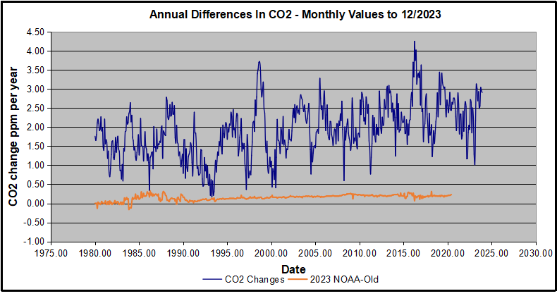
The blue line shows annual observed differences in monthly values year over year, e.g. June 2020 minus June 2019 etc.  The first 12 months (1979) provide the observed starting values from which differentials are calculated.  The orange line shows those CO2 values changed slightly in the 2020 dataset vs. the 2014 dataset, on average +0.035 ppm.  But there is no pattern or trend added, and deviations vary randomly between + and -.  So last year I took the 2020 dataset to replace the older one for updating the analysis.

Now I find the NOAA dataset starting in 2021 has almost completely new values due to a method shift in February 2021, requiring a recalibration of all previous measurements.  The new picture of ΔCO2 is graphed below.

The method shift is reported at a NOAA Global Monitoring Laboratory webpage, Carbon Dioxide (CO2) WMO Scale, with a justification for the difference between X2007 results and the new results from X2019 now in force.  The orange line shows that the shift has resulted in higher values, especially early on and a general slightly increasing trend over time.  However, these are small variations at the decimal level on values 340 and above.  Further, the graph shows that yearly differentials month by month are virtually the same as before.  Thus I redid the analysis with the new values.

Global Temperature Anomalies (ΔTemp)

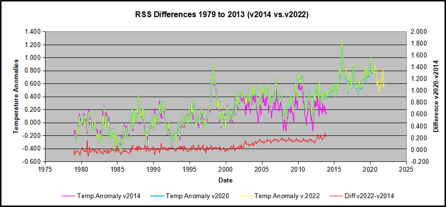
The other time series was the record of global temperature anomalies according to RSS. The current RSS dataset is not at all the same as the past.

Here we see some seriously unsettling science at work.  The purple line is RSS in 2014, and the blue is RSS as of 2020.  Some further increases appear in the gold 2022 rss dataset. The red line shows alterations from the old to the new.  There is a slight cooling of the data in the beginning years, then the three versions mostly match until 1997, when systematic warming enters the record.  From 1997/5 to 2003/12 the average anomaly increases by 0.04C.  After 2004/1 to 2012/8 the average increase is 0.15C.  At the end from 2012/9 to 2013/12, the average anomaly was higher by 0.21. The 2022 version added slight warming over 2020 values.

RSS continues that accelerated warming to the present, but it cannot be trusted.  And who knows what the numbers will be a few years down the line?  As Dr. Ole Humlum said some years ago (regarding Gistemp): “It should however be noted, that a temperature record which keeps on changing the past hardly can qualify as being correct.”

Given the above manipulations, I went instead to the other satellite dataset UAH version 6. UAH has also made a shift by changing its baseline from 1981-2010 to 1991-2020.  This resulted in systematically reducing the anomaly values, but did not alter the pattern of variation over time.  For comparison, here are the two records with measurements through December 2023.

Comparing UAH temperature anomalies to NOAA CO2 changes.

Here are UAH temperature anomalies compared to CO2 monthly changes year over year.

Changes in monthly CO2 synchronize with temperature fluctuations, which for UAH are anomalies now referenced to the 1991-2020 period.  As stated above, CO2 differentials are calculated for the present month by subtracting the value for the same month in the previous year (for example June 2022 minus June 2021).   Temp anomalies are calculated by comparing the present month with the baseline month.

The final proof that CO2 follows temperature due to stimulation of natural CO2 reservoirs is demonstrated by the ability to calculate CO2 levels since 1979 with a simple mathematical formula:

For each subsequent year, the co2 level for each month was generated

CO2  this month this year = a + b × Temp this month this year  + CO2 this month last year

Jeremy used Python to estimate a and b, but I used his spreadsheet to guess values that place for comparison the observed and calculated CO2 levels on top of each other.

In the chart calculated CO2 levels correlate with observed CO2 levels at 0.9986 out of 1.0000.  This mathematical generation of CO2 atmospheric levels is only possible if they are driven by temperature-dependent natural sources, and not by human emissions which are small in comparison, rise steadily and monotonically.

Comment:  UAH dataset reported a sharp warming spike starting mid year, with causes speculated but not proven.  In any case, that surprising peak has not yet driven CO2 higher, though it might,  but only if it persists despite the likely cooling already under way.

Previous Post:  What Causes Rising Atmospheric CO2?

nasa_carbon_cycle_2008-1

This post is prompted by a recent exchange with those reasserting the “consensus” view attributing all additional atmospheric CO2 to humans burning fossil fuels.

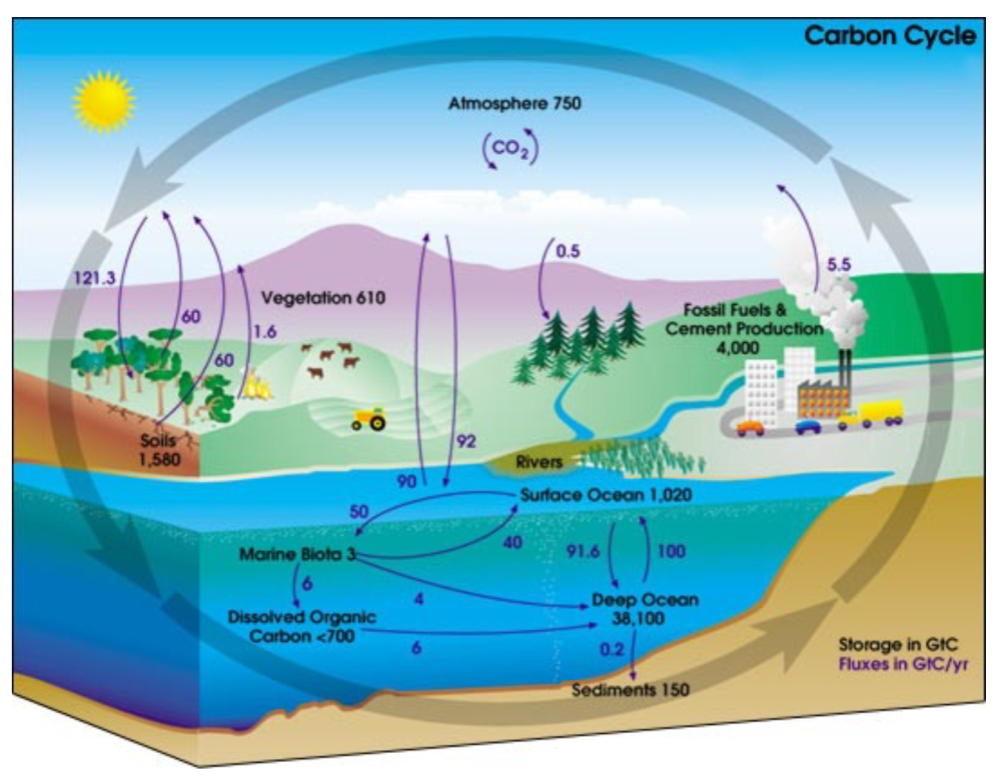
The IPCC doctrine which has long been promoted goes as follows. We have a number over here for monthly fossil fuel CO2 emissions, and a number over there for monthly atmospheric CO2. We don’t have good numbers for the rest of it-oceans, soils, biosphere–though rough estimates are orders of magnitude higher, dwarfing human CO2.  So we ignore nature and assume it is always a sink, explaining the difference between the two numbers we do have. Easy peasy, science settled.

What about the fact that nature continues to absorb about half of human emissions, even while FF CO2 increased by 60% over the last 2 decades? What about the fact that in 2020 FF CO2 declined significantly with no discernable impact on rising atmospheric CO2?

These and other issues are raised by Murray Salby and others who conclude that it is not that simple, and the science is not settled. And so these dissenters must be cancelled lest the narrative be weakened.

The non-IPCC paradigm is that atmospheric CO2 levels are a function of two very different fluxes. FF CO2 changes rapidly and increases steadily, while Natural CO2 changes slowly over time, and fluctuates up and down from temperature changes. The implications are that human CO2 is a simple addition, while natural CO2 comes from the integral of previous fluctuations.  Jeremy Shiers has a series of posts at his blog clarifying this paradigm. See Increasing CO2 Raises Global Temperature Or Does Increasing Temperature Raise CO2 Excerpts in italics with my bolds.

The following graph which shows the change in CO2 levels (rather than the levels directly) makes this much clearer.

Note the vertical scale refers to the first differential of the CO2 level not the level itself. The graph depicts that change rate in ppm per year.

There are big swings in the amount of CO2 emitted. Taking the mean as 1.6 ppmv/year (at a guess) there are +/- swings of around 1.2 nearly +/- 100%.

And, surprise surprise, the change in net emissions of CO2 is very strongly correlated with changes in global temperature.

This clearly indicates the net amount of CO2 emitted in any one year is directly linked to global mean temperature in that year.

For any given year the amount of CO2 in the atmosphere will be the sum of

  • all the net annual emissions of CO2
  • in all previous years.

For each year the net annual emission of CO2 is proportional to the annual global mean temperature.

This means the amount of CO2 in the atmosphere will be related to the sum of temperatures in previous years.

So CO2 levels are not directly related to the current temperature but the integral of temperature over previous years.

The following graph again shows observed levels of CO2 and global temperatures but also has calculated levels of CO2 based on sum of previous years temperatures (dotted blue line).

Summary:

The massive fluxes from natural sources dominate the flow of CO2 through the atmosphere.  Human CO2 from burning fossil fuels is around 4% of the annual addition from all sources. Even if rising CO2 could cause rising temperatures (no evidence, only claims), reducing our emissions would have little impact.

Atmospheric CO2 Math

Ins: 4% human, 96% natural
Outs: 0% human, 98% natural.
Atmospheric storage difference: +2%
(so that: Ins = Outs + Atmospheric storage difference)

Balance = Atmospheric storage difference: 2%, of which,
Humans: 2% X 4% = 0.08%
Nature: 2% X 96 % = 1.92%

Ratio Natural:Human =1.92% : 0.08% = 24 : 1

Resources
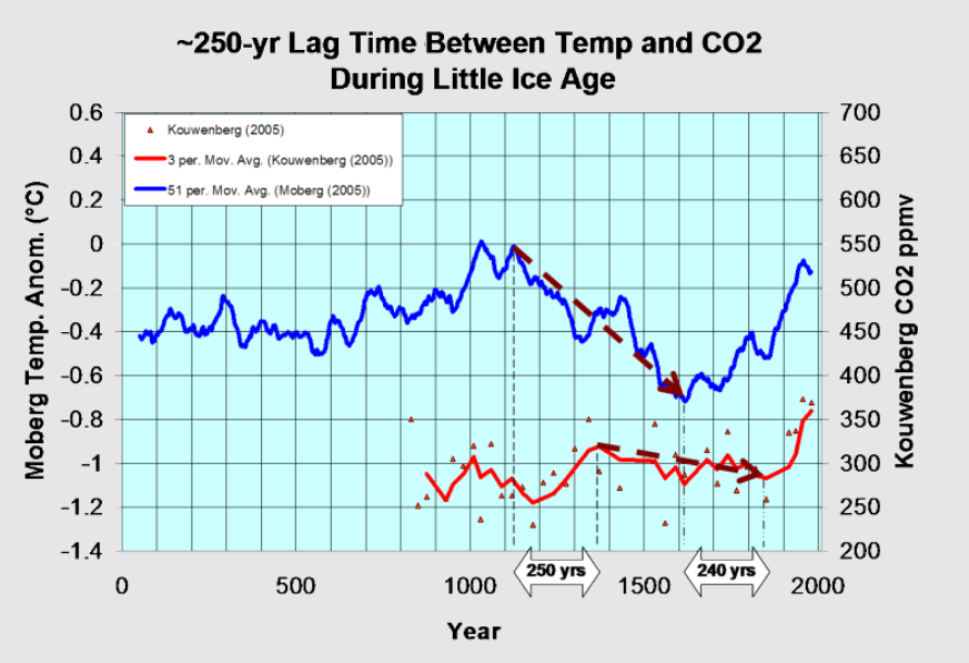
For a possible explanation of natural warming and CO2 emissions see Little Ice Age Warming Recovery May be Over
Resources:

CO2 Fluxes, Sources and Sinks

Who to Blame for Rising CO2?

Fearless Physics from Dr. Salby

via Science Matters

https://ift.tt/zkuTscB

January 7, 2025 at 10:47AM

EV Sales Still Way Below Target

By Paul Homewood


 image

https://www.smmt.co.uk/vehicle-data/car-registrations/

SMMT have released the final data for car registrations last year. BEVs ended the year with a market share of 19.6%, well below the ZEV mandate of 22%, despite a bumper December.

BEV registrations for the month were 56% compared to December 2023, which clearly is not a representative figure. Remember that these are registrations, not sales. It is therefore extremely likely that carmakers have been pre-registering thousands of EVs, in order to get closer to their target. We also know they have been offering unaffordable discounts for purchases before the end of the year.

Either way, there appears to be no way that BEV share will rise to the mandated 28% this year.

It is worth looking behind the numbers though.

First of all, EV take up in the private sector remains stubbornly low at one-in-ten. There is simply no way total EV sales will get anywhere target if private buyers, who account for 38% of the market, refuse to buy them.

image

https://www.smmt.co.uk/2025/01/record-ev-market-share-but-weak-private-demand-frustrates-ambition/

.

Secondly sales of petrol and diesels fell sharply in December, as carmakers cut back on production, in order to artificially raise the ratio of EVs.

This is evident from the November manufacturing figures, which are 30% down on November 2023.


image

https://www.smmt.co.uk/2024/12/car-manufacturing-down-in-november-as-sector-seeks-an-easing-of-cost-pressures/

Registration of Ford cars last year in the UK fell by 23%, Nissan 12%, Toyota 8% and Vauxhall 21%. These are alarming figures, not least for the two Japanese companies.

Nissan, for instance, saw registrations fall from 100K to 89K between 2023 and 2024. Sales of the Leaf have been plummeting recently, and sales of the petrol/diesel Qashqai and Juke models account for 77K on their own. Clearly Nissan will miss the 22% target by a long way.

So will Toyota, who have been been specialising in hybrids in recent years. Late to the EV party, their only electric offering, the Toyota bZ4X, was only introduced to the UK last June, and costs over £40,000, well outside the affordability of the mass market sector. Toyota registrations fell from 108K to 101K last year. Expect more large cutbacks next year to reduce sales of petrol/diesel.

Neither Nissan or Toyota are in strong position to meet the challenge of Chinese made EVs, and there surely must be question marks over their future UK operations, as they will no longer be viable under existing ZEV mandates.

Meanwhile Chinese EV manufacturers, Polestar and BYD, clocked up 17481 EV registrations in 2024, giving them 13635 surplus ZEV allowances, which they may be able sell at a price close £15000 each to carmakers who have fallen short of target and will otherwise have to pay that much in fines. That will hand Polestar and BYD a nice little windfall of £204 million!

Tesla too will rubbing their hands with glee, with their 50334 registrations, potentially worth £600 million.

If you wanted to destroy the UK car industry, while enriching Chinese and US manufacturers, I cannot think of a better way to do it!

via NOT A LOT OF PEOPLE KNOW THAT

https://ift.tt/NH7dI1W

January 7, 2025 at 09:10AM

Wednesday

0 out of 10 based on 0 rating

via JoNova

https://ift.tt/DW9ToVU

January 7, 2025 at 09:01AM